The Effect of the 2008 Financial Crisis on Bosnian Households
1 Introduction
Every individual—constantly—is making one of two decisions with their income, to spend it for consumption or save it for future consumption. Unfortunately for us all, individuals can scarcely be certain of their futures, and, in trying to mitigate the risks of an uncertain one, individuals must adjust their consumption-saving behavior. Studying these adjustments broadly is important for understanding how individuals across income levels make decisions, and how those decisions influence the macroeconomy, however, there is limited research in the space covering middle-income countries—in particular, middle-income countries experiencing financial crises. What do people do with their money when they do not know what it will get them tomorrow?
The theory concerning precautionary saving can be traced to the mid-20th century with the permanent income hypothesis (Friedman 1957). Under the permanent income model, individuals anticipate their future incomes with certainty and save in the short run to account for the differences between their present and anticipated incomes. When an individual expects less income in the future, they will save more in the present. In doing this, individuals are smoothing their total consumption across periods rather than riding whatever wave of income is available in a given period. This is beneficial as while some utility from consumption is sacrificed under periods of higher income, it prevents periods of lower income that decrease utility more significantly. Stability across a lifetime is preferable to hopping between relative riches and squalor. In choosing between saving or consuming, one chooses one and forgoes the other today for the benefit of consuming more in the future. When individuals know their futures—as in Friedman’s hypothesis—consumption smoothing is not so tricky, but what if individuals do not know their futures? What if the future is uncertain?
While not the first to consider the effects of uncertainty on saving, an early framework for evaluating those effects can be found in Leland (1968), who constructed a model of precautionary saving, introducing uncertainty to future incomes, and concluded that “[…] saving will be a positive function of uncertainty.” If individuals wish to smooth their consumption but do not know what their future incomes will be, then they do not know how much to save or if to save at all. Without knowing their future incomes, they cannot accurately assess the utility exchange from saving. In fact, individuals at this level can only assess with certainty the utility from consuming their incomes altogether. In this case, individuals are left with two primary approaches: caution or incaution. Individuals may choose to still forgo some consumption in the present and ward off the risk of a poor future period, or to take on the risks of the future. The choice depends on the risk profile of an individual—if individuals have a low or high aversion to risky outcomes. A gambler may be happy to make such a bet, but most people may not be. In the context of a more uncertain future, most individuals will likely become more cautious. Of course, the future is always uncertain, so what makes it more so? What magnitude of event is necessary for a notable change in risk aversion? The exact margin is difficult to assess, but, the 2008 Global Financial Crisis was certainly an event of such magnitude.
In the early 2000s credit availability for home buyers became very broad, resulting in many people who plainly could not afford their homes, buying homes. This availability of credit inflated prices on the housing market through the excess demand generated. Credit must eventually be repaid, however, and to the dismay of lenders, many people who had been lent mortgages for their homes, could not afford to repay. While default among some debtors is not unexpected—in fact, the point of packaging securities with various risk levels was meant to mitigate this—the problem was that many debtors could not pay and that these securities were wrongly rated, understating actual default risk among debtors. A hole thus appeared in all mortgage-related assets as it became clear that a significant amount of value in the housing was essentially hollow. From 2007 to the second quarter of 2011, “[…] home prices fell by over a fifth on average across the nation from the first quarter of 2007 to the second quarter of 2011” (Weinberg 2013). Foreclosure rates ticked up and huge financial institutions teetered under the weight of vapor money, entire market sectors concerned with housing were upended. The crisis in the securities market disrupted the financial system which had depended on the liquidity derived from securities markets. The credit crunch that followed caused the worldwide economic crisis. In response, households became more risk-averse. While the issue was in the housing market, there was a decline in economic activity across the board—people stopped spending as much as they had been. As the crisis worsened, the decline in activity followed and, in all, “[…] US gross domestic product fell by 4.3 percent, making this the deepest recession since World War II” (Weinberg 2013). Even after the recession, the recovery would be lackluster, and it would take years to return to strong growth rates and lower levels of unemployment. Beyond the many households who lost their incomes due to layoffs, many more too actively hesitated to spend money they had out of fear of the recession—thereby prolonging it. The onset of a period of heightened economic uncertainty led American consumers to change their consumption preferences by becoming more risk-averse, ultimately resulting in an even worse downturn than would have otherwise been due to the additional loss in output. This same story played out globally.
Following the 2008 Global Financial Crisis, the theory of precautionary saving has been empirically tested against other national economies. Bande and Riveiro (2013), and Tamura and Matsubayashi (2011) tested the theory against data from the Kingdom of Spain (Spain hereafter) and Japan respectively, both presenting results consistent with theoretical models. The former study comprised a review of Spanish regional data from the late 1980s to the 2010s and the latter covered a similar period in Japan. In the study of Spain, the authors considered a two-period model and found “[…] a significant and positive effect of income uncertainty on saving” with a coefficient of 0.063 (Bande and Riveiro 2013). This finding means that—at least in Spain and according to the authors’ measures of uncertainty—an increase in the level of income uncertainty among households is related to an increase in the proportion of income saved by households. In this study, “[…] uncertainty is the uncertainty measure based on the estimation of the conditional variance of expected future income,” (Bande and Riveiro 2013). Both studies broadly represent the same trends in two different, high-income countries, characterized by an increase in saving under periods of atypical economic uncertainty to limit potential losses in well-being. The risk premium drops for individuals under higher uncertainty. In other words, when people are worried about the future state of the economy, they become more averse to making risky decisions with their own incomes. As noted before, the choice to save or consume under uncertainty depends on how willing individuals are to take on risk. In the case that individuals become less willing, they will save more—the potential gain from consuming in the present is not worth the danger that a risky future presents.
The two works by Bande and Riveiro (2013) and Tamura and Matsubayashi (2011) included changes in consumption-saving behavior under uncertainty in high-income countries. This could mean that these studies’ results are not generalizable to middle-income countries like Bosnia where economic uncertainty can be even more alarming for residents. During the Global Financial Crisis, many deposit holders in Bosnia went as far as to withdraw their money from banks, not just to cover their expenses under a period of belt-tightening, but also to simply keep it as cash under fears of a banking collapse (Dvorsky and Stix 2010). I, therefore, chose to study changes in consumption saving behavior in Bosnia, specifically under the increased uncertainty of the Global Financial Crisis, and apply a well-known economic model, the Ramsey-Cass-Koopmans (RCK) growth model (Cass 1965; Koopmans 1963). The RCK model includes a parameter for risk aversion, \(\theta\), that can be adjusted to account for the appetites of individuals to make risky decisions. I use Bosnian economic data from the Penn World Table (Groningen Growth And Development Centre 2023) and the World Bank covering a period from 1996-2007 to calibrate the model for the Bosnian economy before the financial crisis and then run numerical simulations in Wolfram Mathematica to quantitatively assess the economic effect of an increase in risk aversion. These simulations allow me to isolate the effect of a change in \(\theta\) on the Bosnian economy via simultaneous solutions to functions written following the model, holding other parameters constant.
Per the theory underlying the RCK growth model, I find that the increase in risk aversion results in lower levels of consumption, output, investment, and capital accumulation in the long term. Specifically, I find that between the steady states, output, consumption, and investment decreased by as much as \(2.53\%\), \(2.41\%\), and \(7.40\%\) respectively. In dynamic simulations, I find that at 10 years of transition between the steady states, the growth rate of output decreased by as much as \(0.61\%\), and the growth rates of output, consumption, and investment in that year are \(2.89\%\), \(2.27\%\), and \(0.017\%\) respectively.
In Section 2, I present the theoretical model and results. In Section 3, I calibrate the model according to the macroeconomic ratios derived from the data following Kydland and Prescott (1996). In Section 4, I simulate a change in the coefficient of relative risk aversion and display my steady state and dynamic results. In Section 5, I test the robustness of my results via a sensitivity analysis where I change parameters other than \(\theta\) to see how that impacts my results. In Section 6, I discuss my results and compare them to those of other works.
2 Methodology
2.1 Theoretical Model
A theoretical model describes complex economic processes in simplified terms. Theoretical models do not aim to be perfect representations of an economy but aim to illustrate important relationships. The RCK growth model builds on microeconomic foundations, representing consumption-saving behavior by households and their interactions with firms in a dynamic environment (Cass 1965; Koopmans 1963). I consider the model without debt and deficits but with lump-sum taxes. In the model, households supply their labor and capital to firms in exchange for wages and rents (household income). Additionally, the government provides services for households with revenues raised via their taxing. The money households earn in income (less the amount paid in taxes) is then either put towards consumption—in the contemporaneous period—of the output goods and services produced by those firms or, is saved for consumption of those goods and services in a future period. Table 1 below defines the variables of the theoretical model presented in the next subsections:
| \(\text{Variable}\) | \(~~~~~\text{Description}~~~\) |
|---|---|
| \(\alpha\) | Contribution of Capital to Output (\(\alpha<1\)) |
| \(\theta\) | Coefficient of Relative Risk Aversion (the preferences of individuals to “risk” their incomes towards consumption) |
| \(\rho\) | Rate of Time Preference (the reward for consuming in the immediate period) |
| \(r\) | Interest Rate (the reward for saving) |
| \(n\) | Population Growth Rate |
| \(g\) | Growth Rate of Technological Progress |
| \(k\) | Capital Accumulation |
| \(w\) | Wages |
| \(K\) | Capital Stock |
| \(L\) | Labor |
| \(A\) | Effectiveness of Factors of Production (Capital and Labor) |
| \(T\) | Taxes |
| \(G\) | Government Expenditure |
2.1.1 Firms
The production function of this model is a Cobb-Douglas function where firms operate under perfect competition. The production function is expressed in its intensive form:
\[ Y=F(\frac{K}{AL},1) = f(k) = k^{\alpha} \label{eq:class_eq_1} \tag{1} \]
Profit maximization yields the optimality conditions for wages and the interest rate:
\[ r = f'(k) \label{eq:class_eq_2} \tag{2} \]
\[ w = f(k)-k(f'(k)) \label{eq:class_eq_3} \tag{3} \]
\(\eqref{eq:class_eq_2}\) and \(\eqref{eq:class_eq_3}\) indicate that the interest and wage rates correspond to the marginal product of capital and labor respectively.
2.1.2 Households
Households make decisions to save or consume, considering future periods as well as the present, and their consumption-saving behavior is characterized by constrained utility maximization. Households want to maximize their utility across periods and into the future according to their risk and rate of time preferences. The coefficient of relative risk aversion defines the risk preferences of households and is expressed as:
\[ \theta=\frac{-c(u''(c))}{u'(c)} \label{eq:class_eq_4} \tag{4} \]
The constant relative risk aversion (CRRA) utility function takes this coefficient:
\[ u(c(t))=\frac{c(t)^{1-\theta}}{1-\theta} \label{eq:class_eq_5} \tag{5} \]
defining utility according to consumption and risk preferences. Lastly, households maximize their utility according to the CRRA and their rate of time preference:
\[ \max{U} = \int_{t=0}^{\infty}e^{-\rho{t}}u(c(t)) dt \label{eq:class_eq_6} \tag{6} \]
The rate of time preference, \(\rho\), illustrates the preferences of households for consuming more in the immediate period. In other words, it is the premium for impatience. While maximizing their utility, households face a dynamic budget constraint:
\[ \dot{k}=(r(t)-n-g)k(t)+w(t)-c(t)-T(t) \label{eq:class_eq_7} \tag{7} \]
which constrains their utility according to how much they can afford, as well as the no-Ponzi-game constraint (Friedman 1957), which restricts households from taking an infinite stream of rolling debt to pay off prior debts. The solution to the problem households face is found via applying the maximum principle on the Hamiltonian function:
\[ \mathscr{H}=\frac{c(t)^{1-\theta}}{1-\theta}+\lambda(t)[r(t)-(n+g)k(t)+w(t)-c(t)] \label{eq:class_eq_8} \tag{8} \]
where \(\lambda(t)\) is marginal utility of consumption. Following the maximum principle, the optimality conditions for households:
\[ \frac{\partial \mathscr{H}(t)}{\partial c(t)}=0 \label{eq:class_eq_9} \tag{9} \]
\[ \frac{\partial \mathscr{H}(t)}{\partial k(t)}=\beta\lambda(t)-\dot{\lambda}(t) \label{eq:class_eq_10} \tag{10} \]
alongside these two is a third, the transversality condition:
\[ e^{-\beta{t}}\lambda(t)k(t)=0 \label{eq:class_eq_11} \tag{11} \]
which says that all capital saved should be put towards consumption by death since individuals can increase utility by increasing consumption (decreasing marginal utility \(\lambda\)) within their lifetimes. In other words, there is no point in saving money you cannot use.
Combining Equations \(\eqref{eq:class_eq_9}\) and \(\eqref{eq:class_eq_10}\) yields the intertemporal allocation of consumption also called the Keynes-Ramsey rule or Euler equation, which describes how households allocate for consumption over time. In per effective worker terms, the Euler equation is:
\[ {\dot{c} \over c}(t)=\frac{1}{\theta}[r(t)-\rho-\theta{(n+g)}] \label{eq:class_eq_12} \tag{12} \]
where \({1 \over \theta}\) represents the elasticity of intertemporal substitution, which describes how much individuals are willing to reallocate consumption across periods of time—and thus how quickly households adjust to new equilibria. A low coefficient of relative risk aversion means a high elasticity of intertemporal substitution, which means that an individual is more willing to reallocate consumption from the present to the future.
2.1.3 Government and General Equilibrium
In this implementation of the RCK model, government spending, \(G(t)\), is financed by lump-sum taxes, \(T(t)\):
\[ G(t) = T(t) \label{eq:class_eq_13} \tag{13} \]
The goods market equilibrium—national accounts identity—closes the model:
\[ Y(t)=C(t)+I(t)+G(t) \label{eq:class_eq_14} \tag{14} \]
By Walras’s law, since the capital and labor markets are in equilibrium, the goods market is also in equilibrium.
2.2 Dynamic and Steady State Equilibria
The dynamic equilibrium is described by the consumption function and dynamic budget constraint equations (loci) respectively:
\[ {\dot{c}}=\frac{1}{\theta}(f'(k)-\rho)-(n+g) \label{eq:class_eq_15} \tag{15} \]
\[ \dot{k}=f(k)-k(n+g)-c-T \label{eq:class_eq_16} \tag{16} \]
and the transversality condition from \(\eqref{eq:class_eq_11}\), which helps to eliminate unstable trajectories. The steady-state equilibrium is achieved whereby \(\dot{c}=\dot{k}=0\), which results in the steady-state equations of the model:
\[ k=({\frac{\theta(n+g)+\rho}{\alpha}})^\frac{1}{\alpha-1} \label{eq:class_eq_17} \tag{17} \]
\[ c=k^{\alpha}-k(n+g)-T \label{eq:class_eq_18} \tag{18} \]
Since \(\alpha<1\), there is a negative exponent meaning that \(\theta\) is at the denominator. This means that an increase in \(\theta\) results in a lower steady-state value of \(k\). Since output, \(y\), is a function of capital, it also results in a lower value of output in the steady state.
Taking all these changes together, the short- and long-run effects of a change in risk aversion can be summarized as follows: In the short run, an increase in \(\theta\) results in a jump in consumption above the prior steady state, although following a decreasing trend with each successive period. In the long run, an increase in \(\theta\) results in capital accumulation, output, and consumption below the steady state. This can be observed in an example phase diagram:
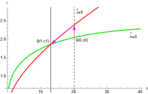
As seen in Figure 1, an increase in \(\theta\) results in the locus for consumption shifting leftward (the dashed black line is the initial steady state and the solid black line is the final steady state), which results in both a lower equilibrium level of consumption and capital accumulation. In the transition between the loci, as seen in arrows on Figure 1, consumption initially spikes in the short-run at \(t=0\) and then drops alongside capital accumulation, in the long run, following the red-colored saddle path of the first locus towards that of the second.
3 Calibration
As per Kydland and Prescott (1996), I calibrate my model. This involves comparing results generated from dynamic simulations with real data. To do this, I use data from the Bosnian economy concerning consumption, investment, government spending, and national income, to create macroeconomic ratios comprised of the former three compared to the latter. I use other data (interest rates, risk aversion, etc.) as parameters for my model, and generate results for consumption, investment, government spending, and national income. I compare the macroeconomic ratios from the real data with those derived from my model and use that comparison to assess the validity of my model.
3.1 Data Description
I source most data on the Bosnian economy from the section covering Bosnia (ordered by country code as “BIH”) in the Penn World Table (Groningen Growth And Development Centre 2023). The data is annual, and observations in the Penn World Table for Bosnia begin in the year 1990 and end in the year 2019. For my data, I am only looking at the period from 1996 to 2007 for the initial steady state, and then the year 2008 for the change in risk aversion, \(\theta\). Data on GDP, \(Y\), is recorded annually in millions at current purchasing power parity (PPP) of 2017 U.S. Dollars (USD). Data on consumption (\(C\)), investment (\(I\)), government spending (\(G\)), and net exports (\(Nx\)), are recorded as decimal shares of GDP that add to one for each year. Consumption as a share of GDP in the Penn World Table includes consumption of both domestic- and foreign-produced goods meaning that the value includes the share from imports, so although my model does not include net exports, I include it in Table 2 to show that the sum of GDP shares add to 1. Data on capital stock, \(K\), is recorded annually at current PPP of 2017 USD. Data on the labor share of GDP (\(wN \over Y\)) is recorded annually. Additional data is collected from the World Bank. Data on the population growth rate, \(n\), is collected from a dataset covering global population growth rates (World Bank 2023). Data on the interest rate, \(r\), is collected from the series on deposit interest rates (World Bank 2024a). The data on the interest rate for Bosnia only began recording observations in 2002. Similarly, data on the tax rate is collected from the series on tax revenue as a percent share of GDP (World Bank 2024c). As with the interest rate, data in the World Bank series only begins recording observations very recently, with the first being in 2005—only three years to use for the average prior to the 2008 crisis. Total factor productivity data is derived via a dataset from Dieppe (2020) that contains values for total factor productivity recorded since 2001 as a percent. This can be used to calculate \(g\) for 2002 and onward by taking the changes between observations1. On the next page is a table listing all data and sources in detail. The Penn World Table and World Bank are abbreviated as “PWT” and “WB” respectively to save space.
| Var. | Description | Source | Link |
|---|---|---|---|
| Y | CGDPo: Output-side real GDP at current PPPs (millions, 2017 USD) | PWT | Link |
| C | Consumption (GDP * csc_h, millions, 2017 USD) | PWT | Link |
| G | Government Spending (GDP * csc_g, millions, 2017 USD) | PWT | Link |
| I | Investment (GDP * csc_i, millions, 2017 USD) | PWT | Link |
| Nx | Net Exports (Ex. + Im. = X, millions, 2017 USD) | PWT | Link |
| Ex. | Exports (GDP * csc_x, millions, 2017 USD) | PWT | Link |
| Im. | Imports (GDP * csc_m, millions, 2017 USD) | PWT | Link |
| \(C \over Y\) | Share of household consumption at current PPPs | PWT | Link |
| \(I \over Y\) | Share of gross capital formation at current PPPs | PWT | Link |
| \(G \over Y\) | Share of government consumption at current PPPs | PWT | Link |
| \(Ex. \over Y\) | Share of goods exports at current PPPs | PWT | Link |
| \(Im. \over Y\) | Share of goods imports at current PPPs | PWT | Link |
| \(\epsilon \over Y\) | Share of residual trade and GDP statistical discrepancy at current PPPs | PWT | Link |
| \(n\) | Population Growth (Annual, %) | WB | Link |
| \(g\) | Total Factor Productivity (Annual, log diff. %) | WB | Link |
3.2 Parameters and Model Economy
3.2.1 Parameters for the Initial Economy
I first find the average values for consumption, investment, government expenditure, net exports, and labor as a share of GDP over the 11-year period from 1996 (the first year after the Bosnian War) to 2007 (the last year before the 2008 crisis). These values are the representation of the initial steady state for the actual economy.
I derive my initial parameters from those macroeconomic ratios and the equations of the model. The equilibrium condition for the wage rate described in Section 2.1.1 gives the following formula for \(\alpha\):
\[ \alpha=1-\frac{wN}{Y} \label{eq:class_eq_19} \tag{19} \]
which solves for \(\alpha\), the contribution of capital to output according to the contribution of labor to output. I solve for its value using the average of \(wN \over Y\) over a period from 1996 to 2007 and choose a value slightly below the solution. I choose a value below the solution, \(\alpha = {1 \over 3}\) so that Wolfram Mathematica cooperates. For \(n\) (the population growth rate), I take the average growth rate of the population over a period from 1996 to 2007 using World Bank data. The data on population growth is heavily skewed by the war in the 1990s with a positive average prior to 2008. In reality, the population has been steadily declining for decades and there are 1 million fewer persons in Bosnia today than in 1996. The reason that the average value for \(n\) prior to 2008 is positive is because the World Bank data asserts that the growth rate of the Bosnian population was \(4\%\) in 1996. This I believe to be from repatriations and better record-keeping post-war. The Penn World Table offers population data as well (Groningen Growth And Development Centre 2023), but using that instead would result in problems that I will detail later. For \(g\) (the growth rate of technological progress), I take the average of the change in total factor productivity from 2002 to 2007. For \(T \over Y\) (the exogenous ratio of taxes to output), I take the average tax revenue as a percentage of GDP from 2005 to 2007. It is assumed in the model that government taxation equals government expenditure, \(G\). For \(\rho\) (the rate of time preference), I take the average deposit rate, r, over a period from 2002 to 2007 to calibrate the rate of time preference. I take an average because I want to know what the deposit rate generally was in the period prior to 2008. The rate of time preference is a parameter within the continuous function seen in Equation \(\eqref{eq:class_eq_6}\) that can be related to the interest rate (a discrete-time variable). More specifically, if the interest rate is the price of time passing, the rate of time preference is the discount for getting things immediately. If the interest rate is higher, individuals place a greater discount on immediate prices.
For the initial coefficient of relative risk aversion, I take the estimate of \(\theta = 0.72\) found by authors Gándelman and Hernández-Murillo (2015). This estimate is in line with those of similar middle-income countries from the paper in the same period. Additionally, the average value for the rate of time preference (\(\rho=0.03776\)) obtained using the deposit interest rate is comparable to that (\(\rho=0.03678\)) which is achieved using a formula based on the Euler equation expressed in the steady state. This formula is expressed as:
\[ \theta=\frac{(r-\rho)}{(n+g)} \label{eq:class_eq_20} \tag{20} \]
and is rewritten to solve for the rate of time preference, with the average (prior to 2008) values of the deposit interest rate, population growth rate, and growth rate of technological progress alongside \(\theta = 0.72\) plugged in:
\[ \rho = r - \theta(n + g) \label{eq:class_eq_21} \tag{21} \]
As noted previously, the rate of time preference illustrates the preferences of households for consuming more in the immediate period. Equation \(\eqref{eq:class_eq_20}\) describes risk aversion in terms that include the rate of time preference subtracting the interest rate. Rewriting this, Equation \(\eqref{eq:class_eq_21}\) describes the rate of time preference in terms of risk aversion—adjusted by the growth rates of population and technological progress—subtracting from the interest rate. The higher the interest rate or lower the coefficient of relative risk aversion, the higher the rate of time preference—the premium for getting things sooner is higher when you are less concerned about risks. Of course, it is worth recalling that the rate of time preference is also a function of the interest rate alone. The resulting values from each method are close, which further evidences this to be a reasonable estimate for the initial coefficient of relative risk aversion.
In the steady state, my model underestimates the ratio of consumption, (greatly underestimates) investment and government expenditure to output:
| Bosnia | \(~~~~~\frac{C}{Y}~~~\) | \(~~~~~\frac{I}{Y}~~~\) | \(~~~~~\frac{G}{Y}~~~\) | \(~~~~~\frac{Nx}{Y}~~~\) |
|---|---|---|---|---|
| Actual Economy | \(~~~~0.8390~~~\) | \(~~~~0.2151~~~\) | \(~~~~0.2546~~~\) | \(-0.3024~~~\) |
| Model Economy | \(~~~~0.7704~~~\) | \(~~~~0.0197~~~\) | \(~~~~0.2099~~~\) | \(~~~~0~~~\) |
It is worth noting that a significant part of the Bosnian economy is constituted by imports that are not included in this model because it is a closed economy model. This discrepancy leads to the extremely low result for the level of investment in the model economy. We will see however that the dynamic response is more in line with what should be expected. In terms of national accounts, investment is solved for by taking the following difference:
\[ I = Y - C - G - Nx \label{eq:class_eq_22} \tag{22} \]
and in the closed economy model \(Nx=0\):
\[ I = Y - C - G \label{eq:class_eq_23} \tag{23} \]
Equation \(\eqref{eq:class_eq_23}\) should look familiar, as it is the same as the goods market equilibrium from Equation \(\eqref{eq:class_eq_14}\) shown in Section 2.1.3. The issue of the level of investment being underestimated cannot be solved by tweaking other parameters, the model is missing a piece of the puzzle—net exports. Any gains would only go to consumption since investment acts as a residual of output not used towards consumption. For example, because \(T=G\) in the model, it may be assumed from Equation \(\eqref{eq:class_eq_23}\) that a lower value of the exogenous tax ratio parameter (\(T \over Y\)) would lead to higher investment. However, this would ignore that consumption is still solved for first—simultaneously with capital accumulation—and would increase following a decrease in the tax ratio. This means that, in the model, consumption would assume all the gain from a cut in taxes before investment gets the chance to see any of it. Below is a table displaying the steady state were the tax ratio set to \({T \over Y}=0\):
| Bosnia | \(~~~~~\frac{C}{Y}~~~\) | \(~~~~~\frac{I}{Y}~~~\) | \(~~~~~\frac{G}{Y}~~~\) | \(~~~~~\frac{Nx}{Y}~~~\) |
|---|---|---|---|---|
| Actual Economy | \(~~~~0.8390~~~\) | \(~~~~0.2151~~~\) | \(~~~~0.2546~~~\) | \(-0.3024~~~\) |
| Model Economy | \(~~~~0.9803~~~\) | \(~~~~0.0197~~~\) | \(~~~~0~~~\) | \(~~~~0~~~\) |
As seen in Table 3, the resulting share of investment within the model economy is identical to the share found in Table 2, and all gains from the tax cut go to consumption.
Whatever the case, my model estimates the share of consumption in the Bosnian economy quite well, and I move forward with it despite the underestimation of investment. In my dynamic results and sensitivity analysis sections, I will demonstrate that my results are still robust despite this underestimation. Below is the table of parameters for the model presented in the next three subsections:
| \(~~~~~\alpha~~~\) | \(~~~~~\theta~~~\) | \(~~~~~\rho~~~\) | \(~~~~~n~~~\) | \(~~~~~g~~~\) | \(~~~~~{T \over Y}~~~\) |
|---|---|---|---|---|---|
| \(~~~~{1 \over 3}~~~\) | \(~~~~0.72~~~\) | \(~~~~0.03776~~~\) | \(~~~~0.00553~~~\) | \(-0.00320~~~\) | \(~~~~0.20990~~~\) |
3.2.2 Estimation of Change in Risk Aversion Between Steady States
Between steady states, I will be adjusting the value for \(\theta\) to reflect the change in risk aversion. I was unable to similarly find an estimate for Bosnia or a like country immediately following the Global Financial Crisis, meaning that I had to arrive at my own estimation for \(\theta\) for that period. Authors Gándelman and Hernández-Murillo (2015) derived their value (\(\theta=0.72\)) using 2006 Gallup World Poll data and regressing a logarithmic risk utility function2 (\(g\)) on individual self-reports of happiness (\(h\)), income (\(y\)), and a series of controls (\(x\)) with the following model:
\[ g(y)=\begin{cases} \frac{y^{1-\theta}-1}{1-\theta} \text{ if } \theta \ne 1\\ \log(y) \text{ if } \theta=1 \end{cases} \label{eq:HappyPaper1} \tag{24} \]
\[ h_{i} = \alpha + \gamma{g(y_{i})}+x_{i}\beta+v_{i} \label{eq:HappyPaper2} \tag{25} \]
While I would have liked to replicate this methodology given that it produces sound estimates, using Gallup World Poll data was not an option due to the cost involved. Instead, I attempt three different methods of estimation for \(\theta\) in the second period, and I will detail each and their results.
The first method involves solving for \(\theta\) using Equation \(\eqref{eq:class_eq_20}\) with values of the interest and population growth rates, and the growth rate of technological progress, updated for the year 2008. As noted earlier, the population growth rate is positive if derived from the World Bank, and negative if from the Penn World Table over the 1996 to 2007 period. Although the latter appears more reasonable on the surface, \(g\) is also negative, and if both \(n\) and \(g\) are negative, the Equation \(\eqref{eq:class_eq_20}\) returns very wonky (negative) estimates. So, while I acknowledge the real population growth may be negative (although it is fair to say that the conditions of the war make basically any estimate from the era difficult), I cannot use a negative value in the model. Further, \(g\) cannot reasonably be made positive for argument’s sake after being consistently negative for 2008 and the years immediately prior. I therefore resolve to use the averages of \(n\) and \(g\) for the period 1996 to 2008 to account for this issue, allowing \(n\) to remain positive. While it is not ideal, it is more reasonable to say that out of all of the variables involved in Equation \(\eqref{eq:class_eq_20}\), population growth and technological progress rates are the least likely to significantly change in the course of a year absent emergency conditions. I then take the value of the deposit interest rate for 2008, calibrate the rate of time preference as I did with the average prior to 2008 in Section 3.2.1, and plug all the values into Equation \(\eqref{eq:class_eq_20}\). The resulting estimate is \(\theta=1.61\), which is higher than the estimates noted later, but is not unreasonable to see high jumps in risk aversion under the context of the Global Financial Crisis as seen in Bekaert, Engstrom, and Xu (2022).
Although I cannot exactly replicate the methodology of Gándelman and Hernández-Murillo (2015), I can use their essential model \(\eqref{eq:HappyPaper2}\) and substitute it with national rather than individual data. For example, instead of using individual reports of household income, I use per capita Gross Domestic Product. Similarly, rather than using individual reports of happiness, I use the OECD (2017b) Consumer Confidence Index which reflects consumer sentiments nationally. Although data for this index is not available from the OECD for Bosnia, there are a number of countries similar to Bosnia with data available. I choose Greece, Hungary, Slovenia, and Türkiye as they are countries near Bosnia that do not generally have hugely higher incomes (none except Slovenia have a GDP per capita greater than \(\approx\)$20,000 current USD) and have OECD data available. While this is not a one-for-one replacement, these are sets of data that answer alike questions. For income and all other variables—except the Consumer Confidence Index—included in the model \(\eqref{eq:HappyPaper2}\) I find national substitutes for Bosnia covering the period 1996 to 2008. Since not all variables are available monthly, I average the index yearly. Further, since some countries selected from the Consumer Confidence Index do not have data available for many periods prior to 2007 I average the index values for the four countries together yearly. I then regress the model over the period 1996 to 2007 to derive coefficients for each variable. Lastly, I plug in values for the year 2008 and solve for \(\theta\) using the coefficients derived. The substitutes that I was able to find do not change all that much in 2008 relative to the prior years included, so the resulting estimate for \(\theta\) in 2008 is almost equal to that of years prior. Ignoring the limited number of observation periods in this implementation, this method could be useful but the substitute values that I have found simply do not do well by it.
The last estimation method is to take the OECD (2017a) Consumer Barometer, which is the normalized change in the Consumer Confidence Index, and multiply the averaged yearly value for 2008 by the initial estimate (\(\theta =0.72\)). The reasoning for this is that if a measure of happiness can be related to risk aversion—as it is inversely by Gándelman and Hernández-Murillo (2015)—and if the Consumer Confidence Index can be considered a substitute for such a measure, then the change in that index could be considered akin to a change in the prior measure, which would then mean a change in risk aversion. Since this is simply a change value that I am multiplying as a scalar rather than regressing, I am unconcerned by some countries not having data until the 2000s and select a range of values. I select from the four countries (Greece, Hungary, Slovenia, and Türkiye) for the ones with the least (Hungary, \(\Delta \approx -0.06\)) and most (Türkiye, \(\Delta \approx -0.23\)) negative average change in the Consumer Barometer for the year 2008. I also take the average (\(\Delta \approx -0.13\)) across all four countries. This results in three estimates: \(\theta=0.77, 0.81, 0.89\). This is a good range of estimates, although the lowest one is only very marginally different from the initial value. It is worth noting that the low estimate for \(\theta\) comes from the Consumer Barometer for Hungary, which is not considered a middle-income country, whereas the high estimate comes from Türkiye which is considered one. In fact, Türkiye is the only country of the four to be considered middle-income, so perhaps the higher estimate is a better characterization for Bosnia. To support this, looking at another middle-income country—albeit one not close to Bosnia—Brazil has an average yearly change that is more negative than the average of the four countries (\(\Delta \approx -0.17\)). With this in mind, and Bekaert, Engstrom, and Xu (2022), I think it best to focus on the highest estimate, \(\theta=0.89\) of the three.
While the second method would have been ideal, it was not feasible for the reasons outlined earlier. By contrast, the first and third methods each have some positives and negatives. For the former, it provides an estimate that feels sufficiently high given the circumstances while not requiring any particularly severe leaps of logic. However, the first method still requires me to hold constant some data that is not constant—even if it is slow-changing—and to make personal assumptions about data integrity under wartime conditions. For the latter, it requires only the assumption that consumer confidence and happiness are closely related. However, the third method provides much lower estimates than the first—not even the largest one is two-tenths greater than the pre-crisis estimate—and frankly, the numbers appear too low for a financial crisis based on analyses of changes in risk-aversion during the financial crisis (Bekaert, Engstrom, and Xu 2022). In all, I carry forward the former and latter as the high and low ends of a range of possible estimates. I also take the mean of the two \(\theta=1 .25\) to serve as a middle-road estimate.
| \(~~~~\text{Low}~~~\) | \(~~\text{Middle}~~~\) | \(~~~~\text{High}~~~\) | |
|---|---|---|---|
| \(~~~~\theta~~~\) | \(~~~~0.89~~~\) | \(~~~~1.25~~~\) | \(~~~~1.61~~~\) |
4 Results
4.1 Comparative Statics
Comparative statics compares equilibrium steady states following a change in a parameter, other things held constant. Using my three estimates for \(\theta\) in 2008 (0.89, 1.25, 1.61), I calculate three ranges of possible steady states. In the 2008 crisis, Bosnians became more risk-averse, which can be attributed to individuals being less prone to consumption out of fear of an uncertain future. The steady-state table shown below shows the results for all three estimates.
| Steady State | \(~~~~~y~~~\) | \(~~~~~c~~~\) | \(~~~~~i~~~\) |
|---|---|---|---|
| Initial (\(\theta=0.72\)) | \(~~~2.91~~~\) | \(~~~2.24~~~\) | \(~~~0.06~~~\) |
| Final (\(\theta=0.89\)) | \(~~~2.89~~~\) | \(~~~2.23~~~\) | \(~~~0.06~~~\) |
| \(~~~\Delta\) (%) | \(-0.50~~~\) | \(-0.47~~~\) | \(-1.49~~~\) |
| Final (\(\theta=1.25\)) | \(~~~2.86~~~\) | \(~~~2.21~~~\) | \(~~~0.05~~~\) |
| \(~~~\Delta\) (%) | \(-1.53~~~\) | \(-1.45~~~\) | \(-4.52~~~\) |
| Final (\(\theta=1.61\)) | \(~~~2.83~~~\) | \(~~~2.19~~~\) | \(~~~0.05~~~\) |
| \(~~~\Delta\) (%) | \(-2.53~~~\) | \(-2.41~~~\) | \(-7.40~~~\) |
In Table 4, \(\Delta\)(%) represents the change in, output, consumption, and investment between steady states characterized by different values of the coefficient of relative risk aversion, \(\theta\). No matter the higher value of \(\theta\), all variables of interest decrease between steady states—and they decrease more the higher the value of \(\theta\). When \(\theta=0.89\), output, consumption, and investment decrease by \(0.50\%\), \(0.47\%\), \(1.49\%\) respectively. When \(\theta=1.25\), output, consumption, and investment decrease by \(1.53\%\), \(1.45\%\), and \(4.52\%\) respectively. When \(\theta=1.61\), output, consumption, and investment decrease by \(2.53\%\), \(2.41\%\), and \(7.40\%\) respectively. When risk aversion increases by any amount, individuals save more and put less of their incomes towards consumption, but by doing this they decrease output, thus earning less income down the line, resulting in less overall to put towards saving and consumption.
4.2 Dynamics
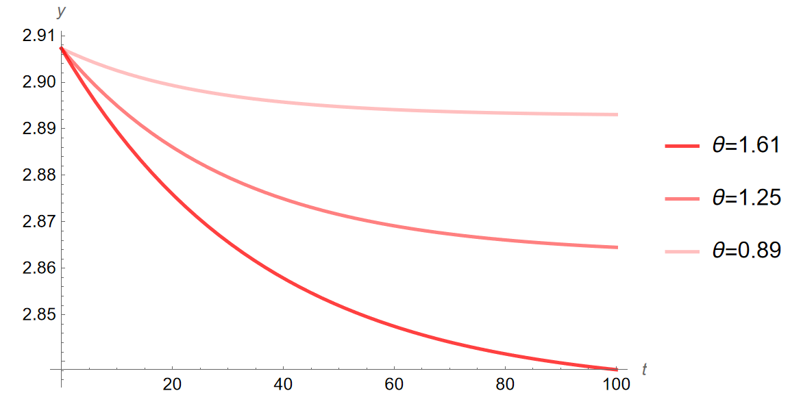
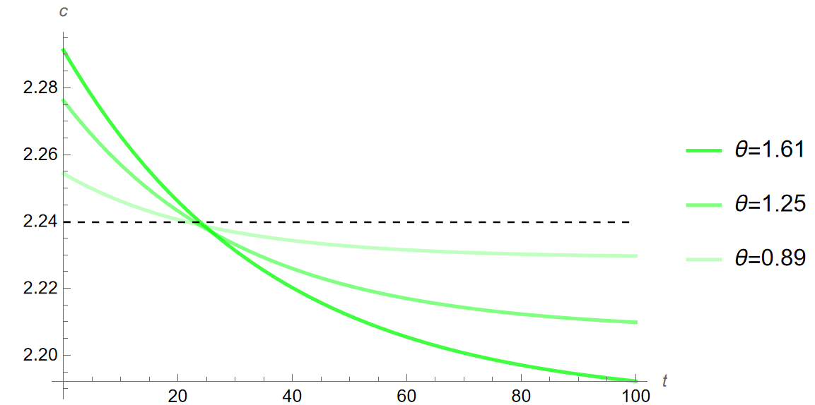
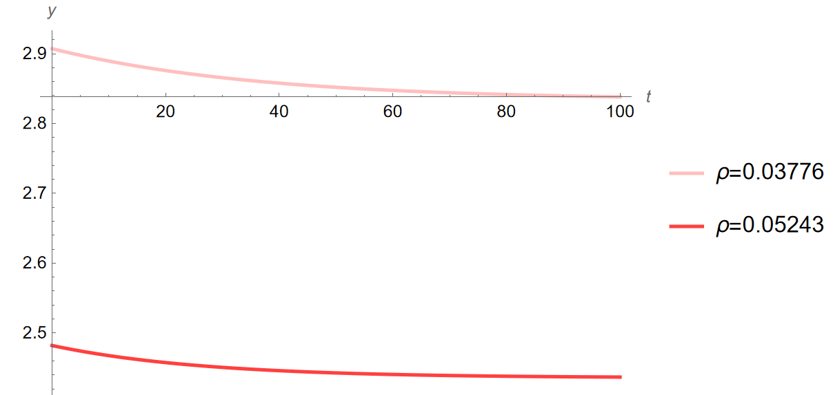
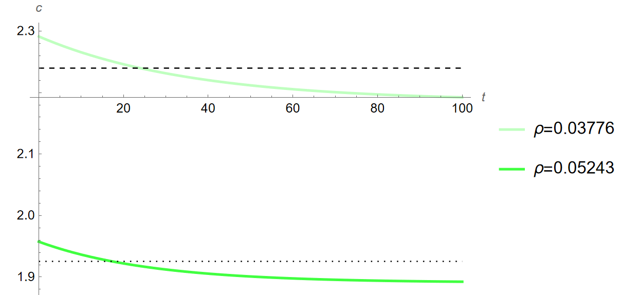
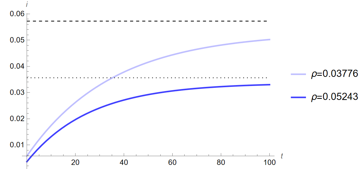
Using the changes in risk aversion outlined previously, I simulate the quantitative impacts on the Bosnian economy of the increase in risk aversion from the 2008 crisis. Below are time paths, graphs illustrating the change in economic variables of interest over time (\(y\), \(c\), \(i\) when \(\theta\) increases from \(0.72\) to \(0.89\), \(1.25\), \(1.61\), \(t=\) years):
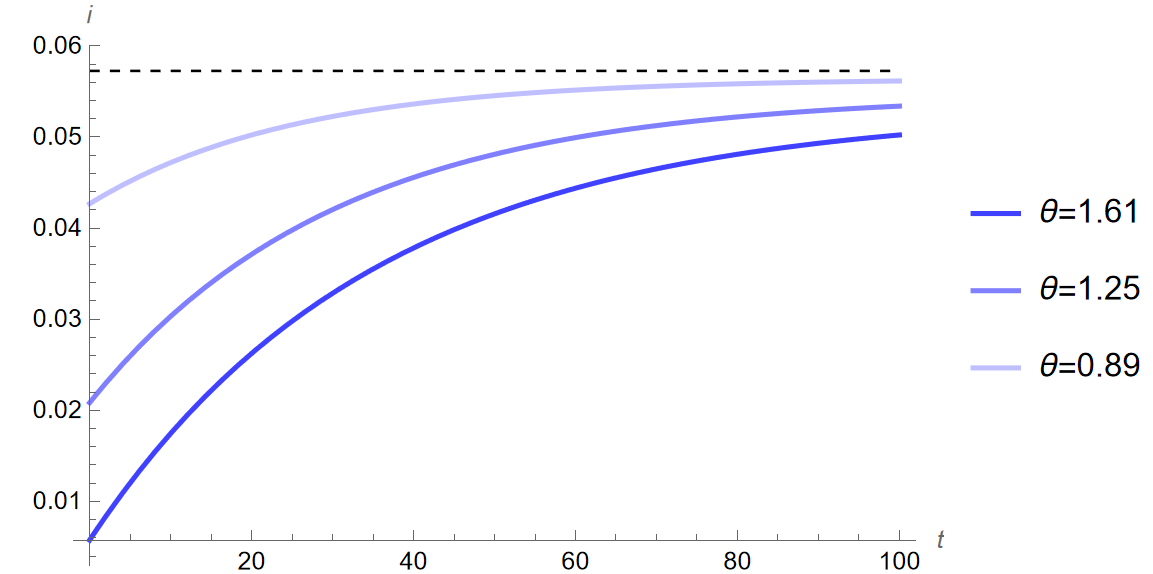
The changes to investment seen in Figure 2 (c) show that the growth rate of investment drops sharply below the steady state and is increasing towards the new equilibrium. By year 100 (\(\theta\) from \(0.72\) to \(1.61\)), investment is only \(12.28\%\) below the steady state. Below are tables showing growth rates by year and the changes in the growth rates illustrating this same dynamic:
| Steady State | Growth Rate | \(~~~~~y~~~\) | \(~~~~~c~~~\) | \(~~~~~i~~~\) |
|---|---|---|---|---|
| \(\theta=0.89\) | On by year 5 | \(~~~2.90~~~\) | \(~~~2.25~~~\) | \(~~~0.05~~~\) |
| On by year 10 | \(~~~2.90~~~\) | \(~~~2.25~~~\) | \(~~~0.05~~~\) | |
| On by year 20 | \(~~~2.90~~~\) | \(~~~2.24~~~\) | \(~~~0.05~~~\) | |
| \(\theta=1.25\) | On by year 5 | \(~~~2.90~~~\) | \(~~~2.27~~~\) | \(~~~0.03~~~\) |
| On by year 10 | \(~~~2.89~~~\) | \(~~~2.26~~~\) | \(~~~0.03~~~\) | |
| On by year 20 | \(~~~2.89~~~\) | \(~~~2.24~~~\) | \(~~~0.04~~~\) | |
| \(\theta=1.61\) | On by year 5 | \(~~~2.90~~~\) | \(~~~2.28~~~\) | \(~~~0.01~~~\) |
| On by year 10 | \(~~~2.89~~~\) | \(~~~2.27~~~\) | \(~~~0.02~~~\) | |
| On by year 20 | \(~~~2.88~~~\) | \(~~~2.25~~~\) | \(~~~0.03~~~\) |
| Steady State | \(\Delta\) in Growth Rate | \(~~~~~y~~~\) | \(~~~~~c~~~\) | \(~~~~~i~~~\) |
|---|---|---|---|---|
| \(\theta=0.89\) | \(\Delta\) by year 5 | \(-0.09~~~\) | \(~~~0.45~~~\) | \(-21.13~~\) |
| \(\Delta\) by year 10 | \(-0.16~~~\) | \(~~~0.28~~~\) | \(-17.58~~\) | |
| \(\Delta\) by year 20 | \(-0.27~~~\) | \(~~~0.03~~~\) | \(-12.28~~\) | |
| \(\theta=1.25\) | \(\Delta\) by year 5 | \(-0.23~~~\) | \(~~~1.16~~~\) | \(-54.65~~\) |
| \(\Delta\) by year 10 | \(-0.43~~~\) | \(~~~0.77~~~\) | \(-47.05~~\) | |
| \(\Delta\) by year 20 | \(-0.73~~~\) | \(~~~0.15~~~\) | \(-35.15~~\) | |
| \(\theta=1.61\) | \(\Delta\) by year 5 | \(-0.33~~~\) | \(~~~1.68~~~\) | \(-78.99~~\) |
| \(\Delta\) by year 10 | \(-0.61~~~\) | \(~~~1.15~~~\) | \(-69.51~~\) | |
| \(\Delta\) by year 20 | \(-1.08~~~\) | \(~~~0.28~~~\) | \(-54.16~~\) |
As seen in Figure 2 across sub-figures Figure 2 (a) through Figure 2 (c) and in Table 6 and Table 5 above, all variables of interest decrease over time following any increase in risk aversion, \(\theta\). Of note is the way each variable of interest changes through time. Output begins at the equilibrium level and decreases with each successive period. By contrast, consumption and investment both begin outside the steady state level at the initial period of change, with consumption beginning above and decreasing thereafter, and investment beginning below and increasing to just below that level by the end. Just as before, based on Equation \(\eqref{eq:class_eq_15}\) and Equation \(\eqref{eq:class_eq_16}\), and the discussion in Section 2.2, it is clear why consumption decreases over time with the change in risk aversion—and since the variables of interest are all related, that explains the changes in the other variables. Consumption decreases because \(\theta\) has increased and \(\theta\) reduces consumption in the steady state equations. Recall that \(1 \over \theta\) represents the elasticity of intertemporal substitution and that if it is low—and with an increase in risk aversion, elasticity would become lower—individuals are more willing to save rather than consume in a single period. Output decreases because it is a function of capital accumulation from the intertemporal budget constraint, and since the capital accumulation decreases to maintain equilibrium when consumption decreases, so does the output. Investment begins below equilibrium and rises to a point still below the initial steady state because it must reflect the national accounts identities as seen in Equation \(\eqref{eq:class_eq_21}\). Since government expenditure is an exogenous constant and this model simulates a closed economy, the only two things that constitute output and can change in terms of national accounts are consumption and investment. Output begins at the equilibrium steady state level and decreases in dynamic simulations, but consumption begins above the steady state and decreases. This means that investment must begin below and rise (although still to a point below equilibrium) for the national accounts identities to hold. These dynamics are consistent with the theory outlined in Section 2.1, and evidence that the model is robust even if it imperfectly estimates the levels.
In the long run, the variables of interest are all below the initial equilibrium level. However, in the earlier periods, consumption is still above the initial steady state, and investment is far below. Looking at Table 6, one can see the changes in the growth rates of the variables over time. By year 10, output and investment are down by \(0.16\%\) and \(17.58\%\) respectively, and consumption is up by \(0.28\%\) when \(\theta=0.89\). However by year 20, output is down by \(0.27\%\) but investment is down by only \(12.28\%\)—indicating that investment is actually increasing back towards the original equilibrium, as seen in Figure 2 (c)—and consumption is up by only \(0.03\%\) when \(\theta=0.89\)—indicating that consumption is decreasing as seen in Figure 2 (b). This same story plays out across all values of \(\theta\). In year 10 when \(\theta=1.25\), output and investment are down by \(0.43\%\) and \(47.05\%\) respectively, and consumption is up by \(0.77\%\), whereas by year 20 output and investment are down by \(0.73\%\) and \(35.15\%\) respectively, and consumption is up by \(0.15\%\). In year 10 when \(\theta=1.61\), output and investment are down by \(0.61\%\) and \(69.51\%\) respectively, and consumption is up by \(1.15\%\), whereas by year 20 output and investment are down by \(1.08\%\) and \(54.16\%\) respectively, and consumption is up by \(0.28\%\). As can be seen, the larger the increase in \(\theta\), the sharper the initial spike and downturn in consumption and investment respectively. Additionally, looking at Table 5, the growth rates of output and consumption are always lowest and investment always highest in year 20 when compared to year 5 respectively, which makes sense given what was observed in Table 6. For example, in year 10 when \(\theta=1.61\), output, consumption, and investment are \(2.89\), \(2.27\), and \(0.02\) respectively, whereas by year 20 output, consumption, and investment are \(2.88\), \(2.25\), and \(0.03\) respectively.
5 Sensitivity Analysis
I introduce three changes: a new value for the rate of time preference, the ratio of taxes to output, and depreciation. I choose these three changes because they all should impact the model in different ways, and seeing if that holds true through dynamic simulations is important to assess the robustness of my results and how sensitive it is to changes in its parameters.
5.1 A New Value of the Rate of Time Preference (\(\rho\))
Recalling the relative roles of the rate of time preference and coefficient of relative risk aversion as the premiums for impatience and patience, and given the increase in the latter between steady states, it is worth investigating the effect of a higher value for the former.
5.1.1 Data and Model
The model does not change with this adjustment. To determine a new value for the rate of time preference (\(\rho\)), I first search for a new value for the interest rate \(r\) and then solve for the value of \(\rho\) as in Section 3.2.1. To find this value, I must change my source of data from the deposit interest rate to something else and take its average. Many typical sources for this rate—bond yields and corporate rates—were not available for the 2007 and prior time periods. I elect to use data on the net interest margin of banks in Bosnia from the World Bank (code: GFDD.EI.01). This records the net interest revenue of banks as a share of their interest-bearing assets, meaning that it illustrates the relative rate of interest banks see yearly. Plugging in the average of values for and before 2007 results in the new value for the rate of time preference, \(\rho=0.05243\). The resulting steady state with the updated value of \(\rho\) shows little change to the estimations of macroeconomic ratios when compared to Table 2.
5.1.2 Results
The variables of interest, \(y\), \(c\), \(i\), all have lower steady-state values with the adjustment to the value of \(\rho\) still decreasing following the changes in \(\theta\) as in the model without the adjusted value of \(\rho\):
| \(~~~~~y~~\) | \(~~~~~c~~\) | \(~~~~~i~~\) | |
|---|---|---|---|
| \(\theta=0.72\) | \(~~~2.91\) | \(~~~2.24\) | \(~~~0.06\) |
| \(\theta=0.89\) | \(~~~2.89\) | \(~~2.23\) | \(~~~0.06\) |
| \(~~~\Delta\) (%) | \(-0.50\) | \(-0.47\) | \(-1.49\) |
| \(\theta=1.25\) | \(~~~2.86\) | \(~~~2.21\) | \(~~~0.05\) |
| \(~~~\Delta\) (%) | \(-1.53\) | \(-1.45\) | \(-4.52\) |
| \(\theta=1.61\) | \(~~~2.83\) | \(~~~2.19\) | \(~~~0.05\) |
| \(~~~\Delta\) (%) | \(-2.53\) | \(-2.41\) | \(-7.40\) |
| \(~~~~~y~~\) | \(~~~~~c~~\) | \(~~~~~i~~\) | |
|---|---|---|---|
| \(\theta=0.72\) | \(~~~2.48\) | \(~~~1.93\) | \(~~~0.04\) |
| \(\theta=0.89\) | \(~~~2.57\) | \(~~~1.92\) | \(~~~0.04\) |
| \(~~~\Delta\) (%) | \(-0.36\) | \(-0.35\) | \(-1.09\) |
| \(\theta=1.25\) | \(~~~2.45\) | \(~~~1.90\) | \(~~~0.03\) |
| \(~~~\Delta\) (%) | \(-1.12\) | \(-1.08\) | \(-3.33\) |
| \(\theta=1.61\) | \(~~~2.44\) | \(~~~1.89\) | \(~~~0.03\) |
| \(~~~\Delta\) (%) | \(-1.86\) | \(-1.80\) | \(-5.49\) |
As seen in Table 7, just as in Table 4, no matter the higher value of \(\theta\), all variables of interest decrease between steady states. When \(\theta=0.89\), output, consumption, and investment decrease by \(0.36\%\), \(0.35\%\), and \(1.09\%\) respectively. When \(\theta=1.25\), output, consumption, and investment decrease by \(2.45\%\), \(1.90\%\), and \(3.33\%\) respectively. When \(\theta=1.61\), output, consumption, and investment decrease by \(1.86\%\), \(1.80\%\), and \(5.49\%\) respectively. However, both the steady-state levels per each value of \(\theta\), and the changes between them are slightly different. Output is decreased in Table 7 (b) (new value of \(\rho\)) when compared to Table 7 (a) (initial \(\rho\)), alongside consumption and investment, but the ratios of the latter two to the former remain about the same as seen when comparing their initial steady states.
Using the new value for the rate of time preference, I simulate the quantitative impacts on the Bosnian economy of the increase in risk aversion from the 2008 crisis. I only simulate the change from \(\theta=0.72\) to \(\theta=1.61\) since the difference in this case is the new value of \(\rho\). Below are time paths comparing the change in the coefficient of relative risk aversion depending on the value of the rate of time preference (\(y\), \(c\), \(i\) when \(\theta\) increases from \(0.72\) to \(1.61\) for when \(\rho\) is \(0.03776\) and \(0.05243\), \(t=\) years):
The dashed and dotted lines in the above figures show the steady state prior to the change in \(\theta\) when \(\rho=0.03776\) and \(\rho=0.05243\) respectively. The time paths of output and consumption are very similar to those seen in Figure 2 (a) and Figure 2, although that of consumption does become negative by year 20. This slight difference in the time path for consumption leads the time path for investment to increase further as time passes. This dynamic of consumption dropping more steeply with time makes sense intuitively: a higher rate of time preference—the premium for impatience—will result in greater emphasis being placed on consumption in earlier years, with later years increasingly written off. These dynamics show that the model is fairly robust.
5.2 A New Value of Taxation (\(T \over Y\))
Given the exogenous nature of the tax ratio, it is worth investigating the effects of changing it in the model. As in Section 3.2.1 when discussing the underestimation of investment in the steady state, government spending takes out a share of GDP in the national accounts identities of Bosnia, but a decrease in it would exclusively go towards a higher steady-state level of consumption. It is worth investigating if there are any other dynamic differences from a change in taxation. By all accounts, there should not be. For this adjustment in the tax ratio, I do not set it to zero, but instead to a slightly higher level. I take the average of government expenditure for the years 2005 to 2007 from the World Bank (2024b) and set the tax ratio to \({T \over Y}=0.34228\). This new value means that over \(34\%\) of output will go towards taxation.
5.2.1 Data and Model
Adjusting the model to simulate the economy with a new value for the tax ratio does not require any changes to it, only to the value of \(T \over Y\).
5.2.2 Results
Only \(c\) has a different—higher— steady-state value when compared to Table 4.
| \(~~~~~y~~\) | \(~~~~~c~~\) | \(~~~~~i~~\) | |
|---|---|---|---|
| \(\theta=0.72\) | \(~~~2.91\) | \(~~~2.24\) | \(~~~0.06\) |
| \(\theta=0.89\) | \(~~~2.89\) | \(~~~2.23\) | \(~~~0.06\) |
| \(~~~\Delta\) (%) | \(-0.50\) | \(-0.47\) | \(-1.49\) |
| \(\theta=1.25\) | \(~~~2.86\) | \(~~~2.21\) | \(~~~0.05\) |
| \(~~~\Delta\) (%) | \(-1.53\) | \(-1.45\) | \(-4.52\) |
| \(\theta=1.61\) | \(~~~2.83\) | \(~~~2.19\) | \(~~~0.05\) |
| \(~~~\Delta\) (%) | \(-2.53\) | \(-2.41\) | \(-7.40\) |
| \(~~~~~y~~\) | \(~~~~~c~~\) | \(~~~~~i~~\) | |
|---|---|---|---|
| \(\theta=0.72\) | \(~~~2.91\) | \(~~~1,85\) | \(~~~0.06\) |
| \(\theta=0.89\) | \(~~~2.89\) | \(~~~1.85\) | \(~~~0.06\) |
| \(~~~\Delta\) (%) | \(-0.50\) | \(-0.47\) | \(-1.49\) |
| \(\theta=1.25\) | \(~~~2.86\) | \(~~~1.83\) | \(~~0.05\) |
| \(~~~\Delta\) (%) | \(-1.53\) | \(-1.44\) | \(-4.52\) |
| \(\theta=1.61\) | \(~~~2.83\) | \(~~~1.81\) | \(~~~0.05\) |
| \(~~~\Delta\) (%) | \(-2.53\) | \(-2.38\) | \(-7.40\) |
The resulting steady state with the updated value of \(T \over Y\) shows no change to investment as a share of GDP, with taxes assuming a portion of the share held prior by consumption. The model now underestimates consumption and still greatly underestimates investment in the steady state. As seen in Table 8, just as in Table 4, no matter the value of \(\theta\), all variables of interest decrease between steady states. When \(\theta=0.89\), output, consumption, and investment decrease by \(0.50\%\), \(0.47\%\), \(1.49\%\) respectively. When \(\theta=1.25\), output, consumption, and investment decrease by \(1.53\%\), \(1.44\%\), and \(4.52\%\) respectively. When \(\theta=1.61\), output, consumption, and investment decrease by \(2.53\%\), \(2.38\%\), and \(7.40\%\) respectively. However, only the steady state levels and changes of consumption are different per each value of \(\theta\) when Table 8 (b) and Table 8 (a) are compared—the levels are the same for output and investment as in Table 4 as well as the changes between steady states. The change to the tax ratio has almost no effect beyond snatching some of the share of output once held by consumption. Unlike the change to \(\rho\) from the prior section, output is not reduced at all by this change to \(T \over Y\), and instead, it is the ratio of consumption to output that is changed, rather than the level of output. This is consistent with Section 3.2.1, where it was demonstrated in Table 3 that changes in taxation only affect consumption in the RCK model.
Using the new value for the tax ratio, I simulate the quantitative impacts on the Bosnian economy of the increase in risk aversion from the 2008 crisis. Below are time paths comparing the change in the coefficient of relative risk aversion depending on the value of the tax ratio (\(y\), \(c\), \(i\) when \(\theta\) increases from \(0.72\) to \(1.61\) for when \(T \over Y\) is \(0.20990\) and \(0.34228\), \(t=\) years):
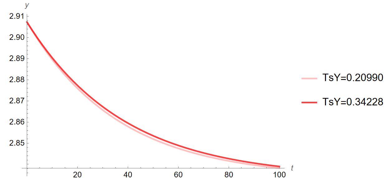
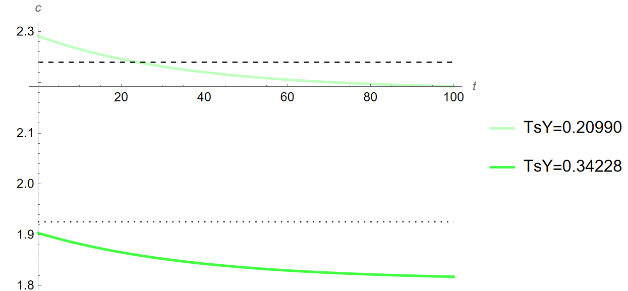
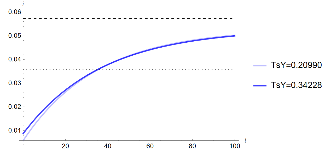
The dashed and dotted lines in the above figures show the steady state prior to the change in \(\theta\) when \({T \over Y}=0.20990\) and \({T \over Y}=0\) respectively. As can be seen, the resulting changes lie entirely with consumption, with it being significantly higher in level at all points in the time path. Do these results imply anything about tax cuts as a policy to stimulate investment? Not really. Again, this is more a reflection of the shortcomings of a closed economy model imposed on an economy with a high trade deficit. However, it is not unreasonable to say that cutting taxes to spur investment would similarly not function as a one-to-one interaction, with much of the difference rather being saved or consumed. Either way, the dynamics of the model are identical following the change in the tax ratio, with consumption only being higher in absolute level. This is consistent with what was discussed in Section 3.2.1, and is further evidence of robustness in terms of dynamic results from the model.
5.3 Introducing Depreciation (\(\delta\))
Given that assets in the real world tend to depreciate, it is worth investigating how introducing a rate of depreciation may impact the model. In the real world, capital depreciation leads to investment in capital stock. Existing machinery, for example, cannot be relied on forever, and must be updated eventually. However, even if introducing depreciation increases the share of investment in output, that share would come from what was held by consumption—taxes are static and exogenous and there are still no trade flows—thus reducing its share of output. However, knowing that these dynamics would be the likely result of the introduction of depreciation to the model, it is worth seeing by how much the shares of each of these things are changed in the steady states and dynamic simulations.
5.3.1 Data and Model
Introducing a non-zero value for depreciation, \(\delta\), adjusts the formulation of the model. The optimality conditions for firms are changed such that Equation \(\eqref{eq:class_eq_2}\) is rewritten as:
\[ r = f'(k)-\delta \label{eq:class_eq_26} \tag{26} \]
which results in new equations of the loci:
\[ \frac{\dot{c}}{c}=\frac{1}{\theta}(f'(k)-\rho)-(\delta+n+g) \label{eq:class_eq_27} \tag{27} \]
\[ \dot{k}=f(k)-k(\delta+n+g)-c-T \label{eq:class_eq_28} \tag{28} \]
and new steady-state equations:
\[ k=({\frac{\theta(\delta+n+g)+\rho}{\alpha}})^\frac{1}{\alpha-1} \label{eq:class_eq_29} \tag{29} \]
\[ c=k^{\alpha}-k(\delta+n+g)-T \label{eq:class_eq_30} \tag{30} \]
Data on the depreciation rate is sourced from the Penn World Table as an average for the 1996 to 2007 period for Bosnia. The resulting steady state with \(\delta\) shows a large change to consumption and investment as shares of GDP. The model now underestimates the share of consumption with the difference being added to the share of investment. This makes sense and follows the theoretical explanation outlined earlier—capital depreciation spurs investment in capital stock, resulting in a larger share of output being diverted to investment.
5.3.2 Results
The steady-state outcomes across values of \(\theta\) show a clear departure from those found in Table 4. While \(y\) and \(c\) are lower across steady states, \(i\) is higher with the non-zero value of \(\delta\).
| \(~~~~~y~~\) | \(~~~~~c~~\) | \(~~~~~i~~\) | |
|---|---|---|---|
| \(\theta=0.72\) | \(~~~2.91\) | \(~~~2.24\) | \(~~~0.06\) |
| \(\theta=0.89\) | \(~~~2.89\) | \(~~~2.23\) | \(~~~0.06\) |
| \(~~~\Delta\) (%) | \(-0.50\) | \(-0.47\) | \(-1.49\) |
| \(\theta=1.25\) | \(~~~2.86\) | \(~~~2.21\) | \(~~~0.05\) |
| \(~~~\Delta\) (%) | \(-1.53\) | \(-1.45\) | \(-4.52\) |
| \(\theta=1.61\) | \(~~~2.83\) | \(~~~2.19\) | \(~~~0.05\) |
| \(~~~\Delta\) (%) | \(-2.53\) | \(-2.41\) | \(-7.40\) |
| \(~~~~~y~~\) | \(~~~~~c~~\) | \(~~~~~i~~\) | |
|---|---|---|---|
| \(\theta=0.72\) | \(~~~1.97\) | \(~~~1.05\) | \(~~~0.51\) |
| \(\theta=0.89\) | \(~~~1.86\) | \(~~~1.04\) | \(~~~0.42\) |
| \(~~~\Delta\) (%) | \(-6.01\) | \(-0.68\) | \(-16.96\) |
| \(\theta=1.25\) | \(~~~1.66\) | \(~~~1.01\) | \(~~~0.30\) |
| \(~~~\Delta\) (%) | \(-15.82\) | \(-3.87\) | \(-40.35\) |
| \(\theta=1.61\) | \(~~~1.52\) | \(~~~0.97\) | \(~~~0.23\) |
| \(~~~\Delta\) (%) | \(-23.09\) | \(-7.80\) | \(-54.50\) |
As seen in Table 9, just as in Table 4, no matter the value of \(\theta\), all variables of interest decrease between steady states. When \(\theta=0.89\), output, consumption, and investment decrease by \(6.01\%\), \(0.68\%\), and \(16.96\%\) respectively. When \(\theta=1.25\), output, consumption, and investment decrease by \(15.82\%\), \(3.87\%\), and \(40.35\%\) respectively. When \(\theta=1.61\), output, consumption, and investment decrease by $23.09%$, $7.80%$, and \(54.50\%\) respectively. However, both the steady-state levels per each value of \(\theta\), and the changes between them are all very different. Introducing depreciation, \(\delta\), greatly reduces the steady-state levels of output and consumption across all values of \(\theta\) and greatly magnifies the size of their changes between steady-state levels. Additionally, the results of investment are very significantly affected by depreciation. The dynamic response of investment is increased ten-fold and decreases sharply between \(\theta\) values. The introduction of depreciation has both reduced output and changed the respective shares of consumption and investment in it. A change in the level makes sense intuitively. First, if assets depreciate output is lost by their depreciation. Second, if assets depreciate, it is necessary to invest in them to prevent further losses to output. Together these two realities explain the level but not the dynamic response.
Using the new value for depreciation, I simulate the quantitative impacts on the Bosnian economy of the increase in risk aversion from the 2008 crisis. Below are time paths comparing the change in the coefficient of relative risk aversion depending on the value of depreciation (\(y\), \(c\), \(i\) when \(\theta\) increases from \(0.72\) to \(1.61\) for when \(\delta\) is \(0\) and \(0.06403~\), \(t=\) years):
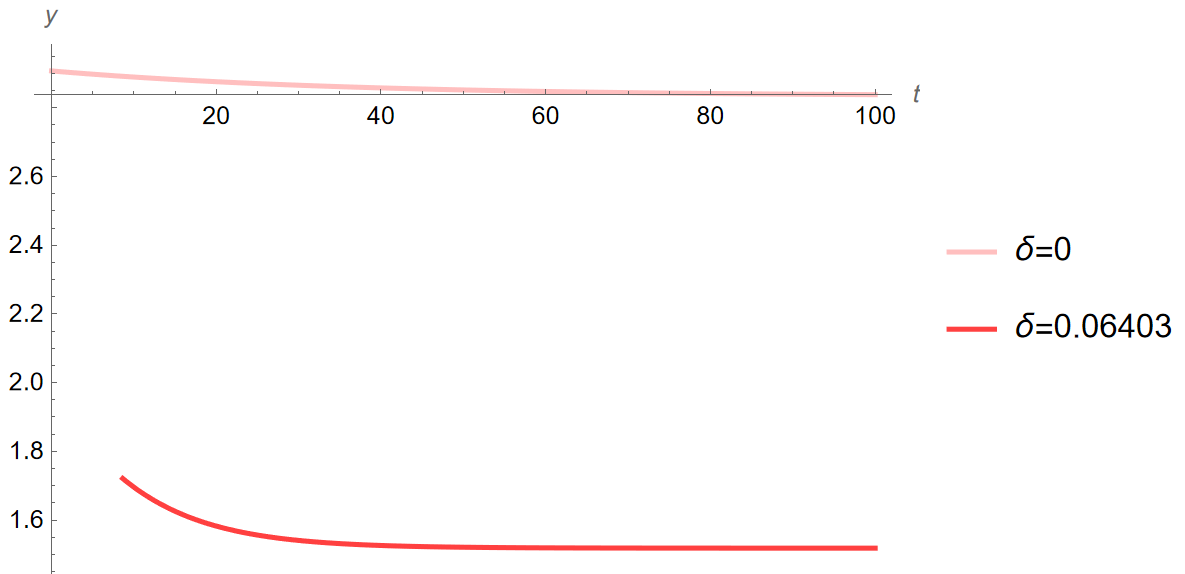
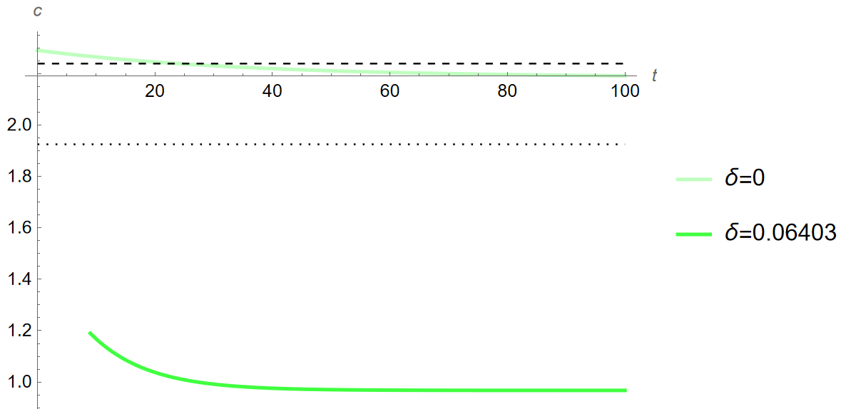
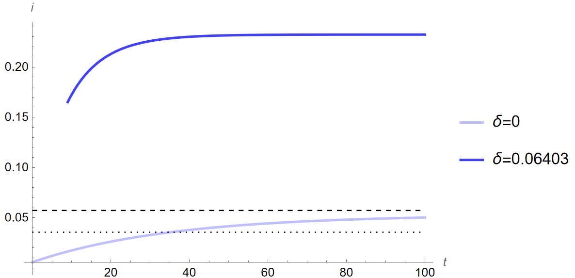
The dashed and dotted lines in the above figures show the steady state prior to the change in \(\theta\) when \(\delta=0\) and \(\delta=0.06403\) respectively. As can be seen, the resulting changes starkly contrast the initial time paths seen in Figure 2. For example, output and consumption begin above their steady states as still expected but decrease so sharply that the first few periods are cut off from the graphs. Investment, by contrast, sees the opposite and is significantly higher across time when compared to Figure 2 (c). The dynamics here are very different from those of the model without depreciation, and evidence that my results with the baseline calibration are not robust to new values of \(\delta\) as far as the dynamic response to investment is concerned.
6 Conclusion
The increase in the coefficient of relative risk aversion, \(\theta\), in Bosnia results in large drops in output, consumption, investment, and capital accumulation. In sum, between the two steady states, output, consumption, and investment, all decrease by as much as \(2.53\%\), \(2.41\%\), and \(7.40\%\) respectively. In dynamic simulations, by year 10, output and investment decrease by as much as \(0.61\%\) and \(-69.51\%\), and the initial spike in consumption is reduced to only \(1.15\%\) over equilibrium when compared to \(1.68\%\) in year 5. As noted in Section 4.2, the changes to investment show that the level of investment drops sharply below the steady state but the growth rate is positively increasing towards the new—still lower—equilibrium. This can be seen in Table 6, where the change to investment in year 5 is even larger in magnitude than in year 10. Additionally, in the sensitivity analysis, all variables of interest still decrease alongside an increase in risk aversion, \(\theta\), although the relative shares fluctuate with the changes in other parameters. The fact that the changes noted from an increase in risk aversion remain consistent through the comparative statics exercise, dynamic simulations, and the sensitivity analysis, except the change to \(\delta\), evidences the model implementation to be robust to changes in the rate of time preference (\(\rho\)) and tax ratio (\(T \over Y\)) but not depreciation (\(\delta\)), and the level of investment in the steady state is underestimated.
Comparing results to Bande and Riveiro (2013) and real-world evidence from Weinberg (2013), I find that the reaction of households to a period of heightened uncertainty in Bosnia resulted in similarly negative adjustments to consumption. In other words, changes to consumption saving behavior in Bosnia, a middle-income country, are comparable to changes in high-income countries. In dynamic simulations with rising levels of risk aversion, individuals reduce their consumption—and, given no alternatives, any income that is not consumed is saved. This reduction in consumption represents a decline in economic activity which results in a decline in output, thereby reducing all macroeconomic variables. This is consistent with the theory outlined by Cass (1965) and Koopmans (1963) and explored in Section 2. This dynamic is noted by Weinberg (2013), who writes that in the real world, output in the United States declined by \(4.3\%\) through the height of the 2008 Global Financial Crisis. My results with the initial parametrization seen in Section 3.2.1 show a decline of \(2.53\%\) at the highest end. It is very well possible that the highest estimate of risk aversion, \(\theta=1.61\), may even be low given how sharp the decline was in the real-world United States and that estimates of risk aversion can range far higher, as seen in Bekaert, Engstrom, and Xu (2022). At the same time, estimating risk aversion at higher levels—particularly given the issues with data availability—runs the risk of overstepping things. Next, although following a different model and methodology, in their consumption growth models, Bande and Riveiro (2013) find the coefficients of their various measures of uncertainty on consumption to range from \(-0.043\) to \(-0.053\), with standard errors ranging from \(1.38\) to \(1.83\). These coefficients from Bande and Riveiro (2013) may appear low in comparison, but that is because they are regression outputs, representing a decrease per one-point increment in their estimates of uncertainty, of which they use multiple and which have ranges of values greater than just one point each. In other words, these are elasticities. Comparing these results to the elasticity of output from the change in risk aversion (\(\theta\) from \(0.72\) to \(1.61\)) in my model implementation:
\[ \frac{(\frac{y_{2}-y_{1}}{y_{1}})}{(\frac{\theta_{2}-\theta_{1}}{\theta_{1}})} \to \frac{(\frac{2.83-2.91}{2.91})}{(\frac{1.61-0.72}{0.72})}=-2.224\% \label{eq:class_eq_31} \tag{31} \]
shows that even an imperfect theoretical model can provide results within the ranges of those like Bande and Riveiro (2013).
Either way, the logic remains the same on both counts—individuals choose to consume less than they would otherwise and in turn experience a loss in utility. As for the spike in consumption in the short run, this is explained by the elasticity of intertemporal substitution (see: Section 2.1.2), which defines how quickly households adjust to new equilibria. Lastly, through the sensitivity analysis, it is clear that the results are robust to changes in parameters other than depreciation and are generally not prone to wild aberrations from their adjustment. The results of my model are therefore broadly in line with conventional theory, evidence from the real world, and prior works.
Given the limited literature covering consumption-saving behavior in Bosnia, more research and data are needed. Time series data on Bosnia does not extend before 1990 in the Penn World Table and the different series from the World Bank have even fewer observations recorded. This data too may be below par in quality for some periods, given the destructive and brutal war that took place during the first half of the 1990-2000 decade, which is why I only included data post-1995 as the Bosnian War ended in December 1995. As for the World Bank data specifically, there are alternative data sources like the Bosnian Agency for Statistics (BHAS) and the Bosnian Central Bank (CBBH) for information on taxation however there are caveats to the data released. Additionally, Bosnia is very dependent on imports and has a significant trade deficit (\(Nx \over Y\) is \(-30\%\)) that clearly impacts its macroeconomic ratios, as discussed in Section 4. This deficit is not totally accounted for in my implementation of the model and an alternative open-economy model could do better by accounting for this discrepancy. Further research could take the form of a more econometric approach like Bande and Riveiro (2013)—which additionally investigates components of uncertainty—or could involve gathering larger sets of data from sources like the BHAS or the CBBH.
7 References
Footnotes
Something worth noting with the Penn World Table data is that it uses a residual/statistical discrepancy variable, “csh_r” to account for disparities in macroeconomic ratios when aggregated over time. Excluding this variable results in macroeconomic ratios that do not add up exactly to 1.↩︎
Gándelman and Hernández-Murillo (2015) use \(\rho\) rather than \(\theta\) for risk aversion but I swapped that to avoid confusion↩︎