The Phillips Curve is Alive and Well in 2023
1 Introduction
The Phillips curve occupies a curious space in post-pandemic economics discourse. While considered “dead” by some, and with some of the strongest evidence for its death coming from the reversal in relationship between inflation and unemployment during that period, it is worth investigating if the issue is the relationship itself, or instead a misspecification of it. Given the significance of both inflation and unemployment concerning economic health, a relationship between the two is an important guide for economic policymakers. To investigate this relationship and how it holds up in 2023, I take quarterly economic data on the United States economy and adopt an econometric variant of the Phillips curve relationship developed by Gordon (2013) and evaluate how well the econometric model matches real values for inflation in the economy. I find that the relationship between unemployment and inflation is indeed still an inverse one, at least in aggregate, with the coefficient on the contemporaneous unemployment gap (unemployment less the natural rate of unemployment) being -0.1097, meaning that the inflation rate is that much lower per 1-point increase in the unemployment gap of the current period. Additionally, I find that the model by Gordon (2013) accurately simulates values for inflation given data from the period.
2 Literature Review
The traditional Phillips curve (traditional curve hereafter) comes from a relationship identified by Bill Phillips between wage pricing and unemployment which was broadened to be defined as one between inflation and unemployment. According to the traditional curve, inflation and unemployment are inversely related—as one goes up, the other goes down. This curve is taught in introductory macroeconomics courses. Given the significance of both inflation and unemployment concerning economic health, the relationship identified between the two took on an important role of its own—a guide for economic policy. Unfortunately for the proud curve (relating two stationary processes), the relationship would not survive the pains of the 1970s.
The 1970s saw a period of stagflation—high inflation conjoined by high unemployment. This was a total reversal in the prior-established relationship of the traditional curve and signaled its weaknesses for the years to come. In response to this change, Robert J. Gordon developed what would become known as the “triangle model” (Gordon et al. 1977; Gordon 1981). In the model, Gordon defines the inflation rate as being dependent on three fundamental elements: underlying inflation, inertia; aggregate demand-pull inflation, demand; and cost push inflation, supply. The first is a lagged rate of inflation, the second is an “[…] index of excess demand” Gordon (1997), which in this case is the unemployment gap, and the third is a number of supply shocks (e.g., food and energy price indices, etc.). For the unemployment gap, Gordon (1997);Gordon (2013) follows the methodology of Staiger, Stock, and Watson (1997) to derive a time-varying natural rate of unemployment (TV-NAIRU hereafter). This method involves regressing lags of the unemployment rate—alongside some supply shock variables depending on who is doing this, Gordon (2013) says excluding shocks for the TV-NAIRU results in better estimates—on the change in inflation, then dividing the intercept coefficient by the coefficients on the lagged unemployment rate regressors and applying a cubic spline. Consider a model where core inflation is regressed on four lags of the unemployment rate:
\[ \pi_{t} = \beta_{0}+\beta_{1}u_{t-1}+\beta_{2}u_{t-2}+\beta_{3}u_{t-3}+\beta_{4}u_{t-4} \label{eq:eq_NAIRU1} \tag{1} \]
where the NAIRU could be derived via Staiger, Stock, and Watson (1997):
\[ \overline{u} = \frac{\beta_{0}}{\beta_{1}+\beta_{2}+\beta_{3}+\beta_{4}} \label{eq:eq_NAIRU2} \tag{2} \]
Doing this over an extended period with a cubic polynomial spline function, one can derive values for the TV-NAIRU through time. Underlying inflation is lagged, demand pull, and cost push inflation can be both contemporaneous and lagged. A simple implementation of the triangle model would be:
\[ \pi_{t} = \beta_{0}+\beta_{1}\pi_{t-1}+\beta_{2}(u_{t}-\overline{u_{t}})+\beta_{3}X_{t} \label{eq:eq_NAIRU3} \tag{3} \]
where Χ is a matrix containing whatever cost push supply shocks are being used. Gordon’s model proved itself to be capable of providing reasonably accurate estimates for inflation, and Gordon himself loves to tout some of the achievements of the triangle model—a prime example: “[…] the model explained in advance in 1982 why the inflation rate fell so rapidly during 1981-86” (Gordon 2013). There are, however, many other variations of the traditional curve. One popular variation is the accelerationist Phillips curve.
The accelerationist Phillips curve (accelerationist curve hereafter) can be traced to Gordon (1968) and takes the relationship of the traditional curve but supplants the unemployment rate with the unemployment gap—just as the triangle model—and the inflation rate with the change in the inflation rate. The change in the inflation rate is derived by simply taking the first differences between periods. Friedman noted that inflation was dependent on inflationary expectations and that individuals’ expectations for inflation were conditioned by past values of it. An implementation of the accelerationist curve could look like (Ball and Mazumder, 2015):
\[ \pi_{t}-\pi_{t-1} = \alpha(u_{t}-\overline{u_{t}})+\epsilon_{t} \label{eq:eq_accel1} \tag{4} \]
rewriting this also helps explain why the triangle model uses inflation as the dependent variable and as regressors rather than a change in inflation:
\[ \pi_{t} = \pi_{t-1}+\alpha(u_{t}-\overline{u_{t}})+\epsilon_{t} \label{eq:eq_accel2} \tag{5} \]
This somewhat resembles the simple form of the triangle model displayed earlier. Although the accelerationist curve was thought up prior to the stagflation of the 1970s, it too—just as the triangle model—does a better job of making sense of that period and the periods to follow than the traditional curve does. Unfortunately, the accelerationist curve does not do as well when presented with inflation and unemployment trends of the late-2000s to early-2010s.
As Gordon (2013) points out, the Phillips curve—including the accelerationist curve (Ball and Mazumder, 2015)—does not do an excellent job at explaining late 2000s inflation. The estimates for inflation, given data on unemployment and prior inflation, should be negative (e.g., we should be seeing deflation according to the traditional and accelerationist curves). This problem is referred to as the missing deflation puzzle as we are seemingly overdue for deflation. Generally, there are two groups with two respective explanations for the missing deflation puzzle (Ball and Mazumder, 2015). James Stock and Robert Gordon (Gordon 2013) say that the problem lay with the unemployment rate being used and argue that the correct specification to solve the missing deflation puzzle would focus on short-term unemployment (e.g., 26 weeks or less) rather than total unemployment. Focusing on short-term rather than total does help explain why “[…] inflation has not fallen by more, because short-term unemployment rose less sharply than total unemployment over 2008-2009 and has since returned to pre-recession levels” (Ball and Mazumder, 2015). Alternatively, other economists argue that the long-standing commitment to a 2% inflation target in the United States has led inflationary expectations to become anchored, preventing “[…] actual inflation from falling very far below that level” (Ball and Mazumder, 2015). But Gordon (2013) also focuses on supply shocks as a crucial factor in modelling inflation and points plainly to the triangle model—whatever the unemployment specification—as a solution to the missing inflation puzzle. This is what most differentiates the triangle model from, say, the accelerationist curve.
The triangle model not only does well in accounting for the trends of the 1970s, but unlike the accelerationist curve also does well in accounting for the trends of the late 2000s. According to Gordon (2013), there is hardly even a deflation puzzle at all, and the problem sits squarely with specifications. In fact, Gordon goes as far as to write “[…] all of the NKPC [New-Keynesian Phillips Curve] literature over the past 15 years, as well as most other research on inflation, fails to include explicit variables to measure the impact of supply shocks. As a result, their misspecified equations attempt to explain the inflation rate that depends on both demand and supply with only a demand variable” (Gordon 2013). Fighting words by the standards of academia—as an aside, simply imagine a respected academic in your field refer to your hard work like this. Regardless, that is how things stood as of 2013.
3 Data
| Variables1 | n | mean | sd | min | max | range | se |
|---|---|---|---|---|---|---|---|
| PCECTPI | 306 | 51.457 | 33.021 | 11.557 | 120.044 | 108.487 | 1.888 |
| JCXFE | 258 | 58.711 | 30.943 | 15.515 | 118.938 | 103.423 | 1.926 |
| UNRATE | 302 | 5.718 | 1.7 | 2.567 | 12.967 | 10.4 | 0.098 |
| ST_UNRATE | 302 | 4.711 | 1.25 | 2.497 | 12.246 | 9.749 | 0.072 |
| OPHNFB | 306 | 62.283 | 26.87 | 23.258 | 115.405 | 92.147 | 1.536 |
The data collected for this paper is sourced primarily from the U.S. Bureau of Economic Analysis (BEA hereafter) and the U.S. Bureau of Labor Statistics (BLS hereafter) via the St. Louis Federal Reserve database (FRED hereafter). The individual datasets are included in the references section, and my compiled datasets are included in the appendix. The FRED stores huge swathes of data from various national and international sources and is dependable. PCECTPI is the Personal Consumption Expenditures index (PCE Headline hereafter), JCXFE is the Personal Consumption Expenditures Less Food and Energy index (PCE Core hereafter), UNRATE is the unemployment rate, ST_UNRATE is the short-term unemployment rate, and OPHNFB is the productivity of nonfarm labor by output per hours worked. The data is quarterly time-series data ending in Q2 2023, with some sets of data being available further back in time than others. Data on the unemployment rate, for example, is available from the BEA as far back as Q1 1948, while PCE Core is only available starting at Q1 1959. All data sourced externally is available by the 1960s and onward. With this in mind, I exclude all data prior to Q1 1960 before making any further changes. I do not end up using short-term unemployment in the triangle model implementation adopted from Gordon (2013) but, I include it with the other data because it is available. I exclude the date variable from the summary statistics tables because it is unnecessary. Below are the summary statistics with the data truncated to Q1 1960 with n = 254 observations for all variables:
| Variables | n | mean | sd | min | max | range | se |
|---|---|---|---|---|---|---|---|
| PCECTPI | 254 | 59.198 | 30.987 | 15.435 | 120.044 | 104.609 | 1.944 |
| JCXFE | 254 | 59.389 | 30.706 | 15.842 | 118.938 | 103.096 | 1.927 |
| UNRATE | 254 | 5.934 | 1.683 | 3.4 | 12.967 | 9.567 | 0.106 |
| ST_UNRATE | 254 | 4.819 | 1.256 | 2.79 | 12.246 | 9.456 | 0.079 |
| OPHNFB | 254 | 69.205 | 24.2 | 32.964 | 115.405 | 82.441 | 1.518 |
All data gathered from the FRED was compiled into a single dataset in R (see appendix: “DATA.R” and “DataCleaned.csv”). The data compiled was transformed to create additional variables (e.g., inflation, differences, changes, moving averages, trends) including a dummy variable, NIXON (subdivided into nixon_price_on and nixon_price_off), that was added to account for the price controls of the Nixon administration using values defined by Gordon (1997);Gordon (2013). Inflation variables are calculated by taking the change between years by quarter in the PCE Core and Headline price indicies. The changes in inflation are calculated by taking the first differences of inflation. The moving averages of inflation are calculated by taking the difference of inflation in one period and the natural logarithm of inflation four quarters prior (Gordon 2013). The food energy effect is the difference between PCE Headline and PCE Core and the food energy effect (late period) is a binary dummy variable where observations prior to 1987 are set to 0 and observations after are equal to the former (Gordon 2013). LT_UNRATE is long-term unemployment and is the difference between UNRATE and ST_UNRATE. The the 8-quarter productivity trend is derived from the 8-quarter percent change in OPHNFB (8-quarter actual productivity) with a Hodrick-Prescott filter (λ = 6400) applied (Gordon 2013). A Hodrick-Prescott filter is useful for just getting the long-run trends of data and Gordon makes effective use of it because of that. This dataset was also compiled in R (see appendix: “DATA.R” and “DataComplete.csv). Below are the summary statistics with the additional variables calculated with the initial data:
| Variables | n | mean | sd | min | max | range | se |
|---|---|---|---|---|---|---|---|
| PCECTPI | 254 | 59.198 | 30.987 | 15.435 | 120.044 | 104.609 | 1.944 |
| Headline π | 254 | 3.306 | 2.43 | -1.196 | 11.514 | 12.71 | 0.152 |
| Headline Δπ | 254 | 0.006 | 0.563 | -2.687 | 2.378 | 5.065 | 0.035 |
| Headline MAπ | 254 | 3.226 | 2.317 | -1.203 | 10.898 | 12.102 | 0.145 |
| JCXFE | 254 | 59.389 | 30.706 | 15.842 | 118.938 | 103.096 | 1.927 |
| Core π | 254 | 3.241 | 2.132 | 0.667 | 10.098 | 9.431 | 0.134 |
| Core Δπ | 253 | 0.01 | 0.359 | -1.436 | 1.698 | 3.133 | 0.023 |
| Core MAπ | 254 | 3.169 | 2.039 | 0.665 | 9.62 | 8.955 | 0.128 |
| Food Energy Effect | 254 | 0.065 | 0.728 | -1.863 | 3.123 | 4.986 | 0.046 |
| Food Energy Effect (Late Period) | 254 | 0.04 | 0.449 | -1.863 | 1.759 | 3.621 | 0.028 |
| UNRATE | 254 | 5.934 | 1.683 | 3.4 | 12.967 | 9.567 | 0.106 |
| ST_UNRATE | 254 | 4.819 | 1.256 | 2.79 | 12.246 | 9.456 | 0.079 |
| LT_UNRATE | 254 | 1.115 | 0.838 | 0.142 | 4.315 | 4.174 | 0.053 |
| OPHNFB | 254 | 69.205 | 24.2 | 32.964 | 115.405 | 82.441 | 1.518 |
| 8-Quarter Prod. Trend | 254 | 4.066 | 1.35 | 2.067 | 6.424 | 4.356 | 0.085 |
| 8-Quarter Actual Prod. | 254 | 4.066 | 2.556 | -1.698 | 10.554 | 12.251 | 0.16 |
| Nixon_price_on | 254 | 0.016 | 0.111 | 0 | 0.8 | 0.8 | 0.007 |
| Nixon_price_off | 254 | 0.013 | 0.142 | 0 | 1.6 | 1.6 | 0.009 |
| NIXON | 254 | 0.028 | 0.179 | 0 | 1.6 | 1.6 | 0.011 |
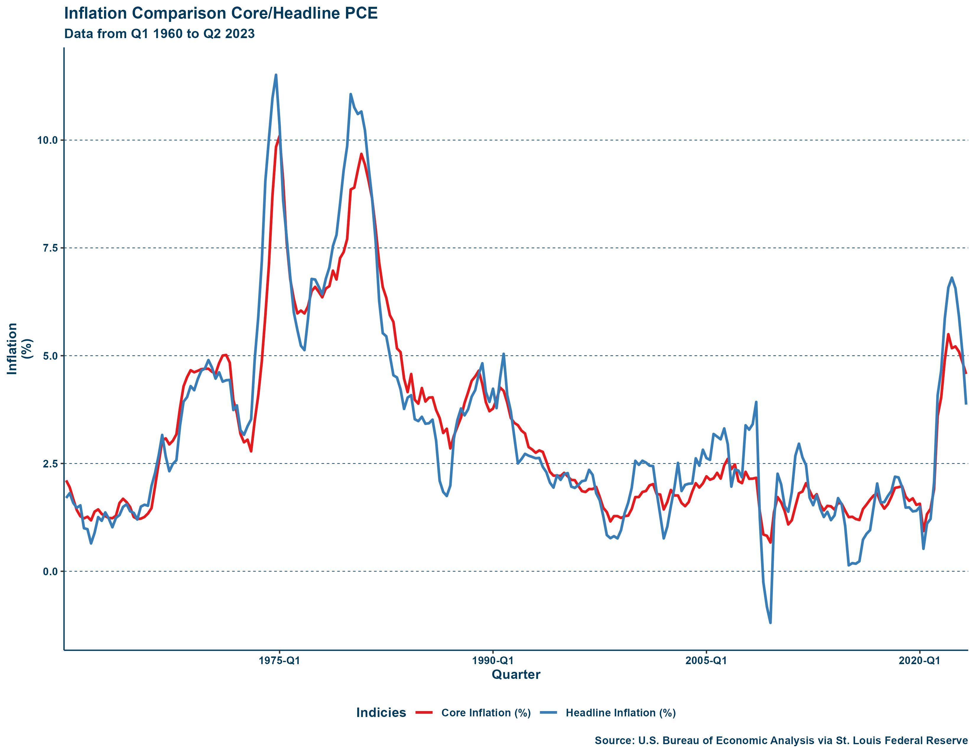
All variables either describe inflation, unemployment, productivity, or some other supply shock. The PCE Core inflation change variable is missing an observation for Q1 1960 but otherwise all variables have observations from then onward. Below is a comparison between Core and Headline PCE:
Lastly, since the accelerationist curve and triangle model use the unemployment gap rather than the unemployment rate, I estimate values for a TV-NAIRU. I create my estimates not by the cubic polynomial spline regression employed by Staiger, Stock, and Watson (1997) and Gordon (1997);Gordon (2013) but instead by running a rolling regression of the unemployment rate on Core PCE inflation. I chose to follow this method under the advice of Professor Sicotte as the alternative spline method was difficult to manage. A rolling regression is easier to implement as it functions as a regular linear model but allows for change over time between periods defined by a “window” of observations. Recalling the earlier regression specification (equation 1) from the literature review, I use the same model but run a rolling regression with a window with a 52-quarter width. I then derive TV-NAIRU estimates according to equation 2 derived from the example by Staiger, Stock, Watson, (1997). The estimates for the TV-NAIRU (NAIRU) achieved by this method are around where one would expect a NAIRU value to be but, the estimates are jagged and change noticeably between individual periods. This is not something wanted from a variable meant to demonstrate long-run trends but luckily this can be resolved by running a Hodrick-Prescott filter (λ = 1600) on the estimates to return smoothed values (NAIRU_smoothed). I then calculate the unemployment gap (UNGAP) by taking the difference between unemployment and the smoothed TV-NAIRU. I also record the unemployment gap using the unsmoothed estimates (UNGAP_raw) just to be thorough, although I do not use them. My method for estimating the TV-NAIRU unfortunately restricts the usable period of data even further to the 1970s and onward as 13 years (52 quarters) of data between the 1960s and 1970s do not have observations for the TV-NAIRU or the unemployment gap. Below is a graph comparing the smoothed and unsmoothed TV-NAIRU values for the unemployment gap:
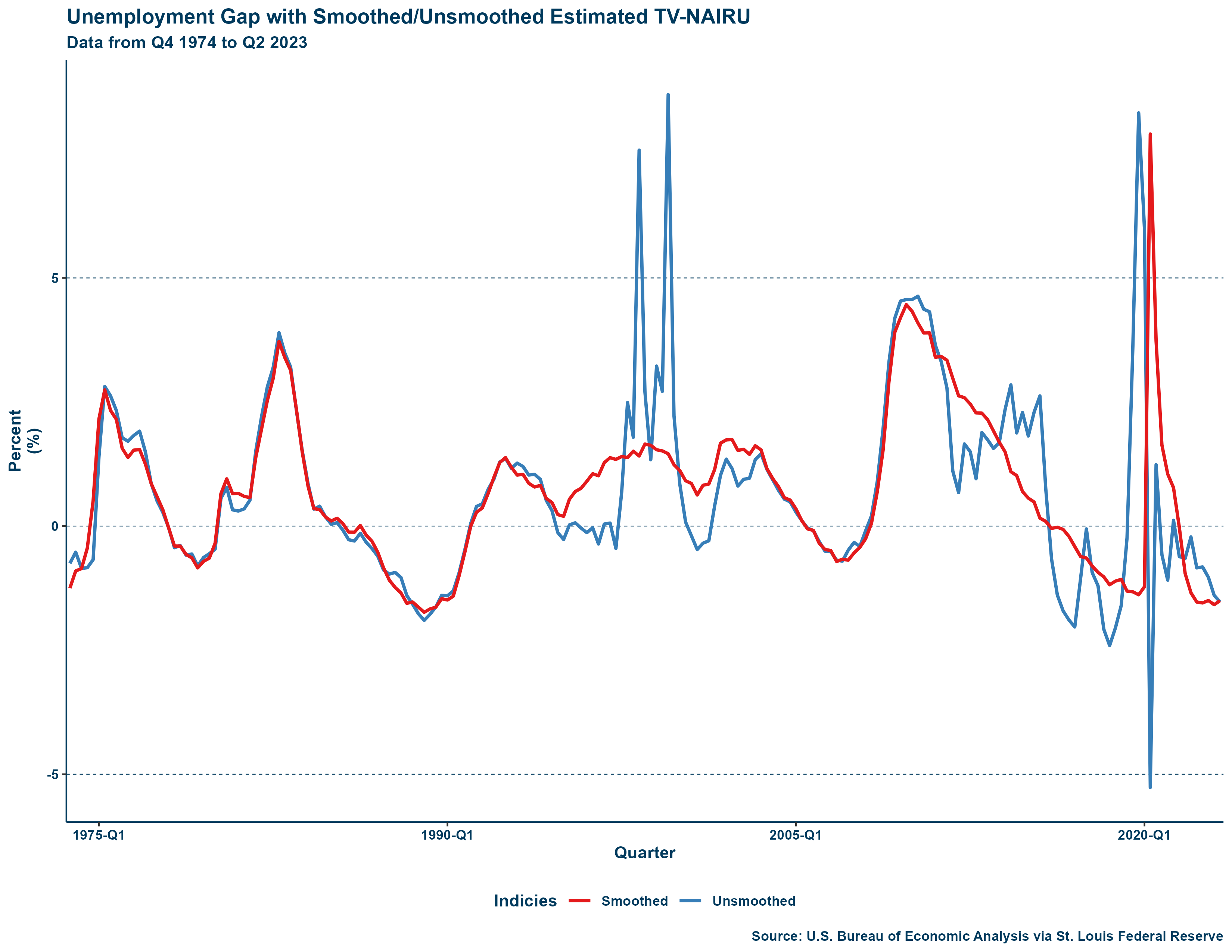
The smoothed unemployment gap is particularly less jagged during the labor market weirdness of the CoVid-19 pandemic which is helpful for the analysis of this paper. This (see appendix: “MODEL.R” and “GordonModelDataset.csv) is the final and complete dataset containing observations for all variables between Q4 1974 and Q2 2023 (n = 199). The summary statistics for this dataset are displayed below:
| Variables | n | mean | sd | min | max | range | se |
|---|---|---|---|---|---|---|---|
| PCECTPI | 199 | 70.62 | 24.903 | 23.11 | 120.044 | 96.934 | 1.765 |
| Headline π | 199 | 3.47 | 2.619 | -1.196 | 11.514 | 12.71 | 0.186 |
| Headline Δπ | 199 | -0.01 | 0.605 | -2.687 | 2.378 | 5.065 | 0.043 |
| Headline MAπ | 199 | 3.38 | 2.493 | -1.203 | 10.898 | 12.102 | 0.177 |
| JCXFE | 199 | 70.704 | 24.682 | 23.474 | 118.938 | 95.464 | 1.75 |
| Core π | 199 | 3.374 | 2.277 | 0.667 | 10.098 | 9.431 | 0.161 |
| Core Δπ | 199 | 0.003 | 0.378 | -1.436 | 1.698 | 3.133 | 0.027 |
| Core MAπ | 199 | 3.295 | 2.176 | 0.665 | 9.62 | 8.955 | 0.154 |
| Food Energy Effect | 199 | 0.096 | 0.786 | -1.863 | 3.123 | 4.986 | 0.056 |
| Food Energy Effect (Late Period) | 199 | 0.051 | 0.507 | -1.863 | 1.759 | 3.621 | 0.036 |
| UNRATE | 199 | 6.208 | 1.732 | 3.5 | 12.967 | 9.467 | 0.123 |
| ST_UNRATE | 199 | 4.929 | 1.343 | 2.79 | 12.246 | 9.456 | 0.095 |
| LT_UNRATE | 199 | 1.278 | 0.867 | 0.345 | 4.315 | 3.97 | 0.061 |
| OPHNFB | 199 | 77.078 | 21.336 | 47.289 | 115.405 | 68.116 | 1.512 |
| 8-Quarter Prod. Trend | 199 | 3.656 | 1.191 | 2.067 | 6.424 | 4.356 | 0.084 |
| 8-Quarter Actual Prod. | 199 | 3.605 | 2.467 | -1.698 | 8.922 | 10.619 | 0.175 |
| Nixon_price_on | 199 | 0 | 0 | 0 | 0 | 0 | 0 |
| Nixon_price_off | 199 | 0.016 | 0.16 | 0 | 1.6 | 1.6 | 0.011 |
| NIXON | 199 | 0.016 | 0.16 | 0 | 1.6 | 1.6 | 0.011 |
| NAIRU_smoothed | 199 | 5.526 | 1.138 | 2.752 | 7.156 | 4.404 | 0.081 |
| NAIRU | 199 | 5.526 | 2.055 | -4.726 | 18.233 | 22.959 | 0.146 |
| UNGAP_raw | 199 | 0.681 | 1.871 | -5.266 | 8.695 | 13.962 | 0.133 |
| UNGAP | 199 | 0.681 | 1.507 | -1.737 | 7.901 | 9.638 | 0.107 |
Many variables (or later lags of these variables) may not be particularly significant, but these are necessary for the replication of the triangle model (Gordon 2013). The only variable not included is the relative price of imports as I simply could not find a source with observations going back far enough to be useful or worthwhile to include.
4 The Curves
As noted before, the traditional curve demonstrates the relationship between the rates of inflation and unemployment. Specifically, the relationship should be an inverse one. Shown below is a graph with a traditional curve constructed by decade with quarterly data from each quarter from Q1 1960 to Q2 2023:
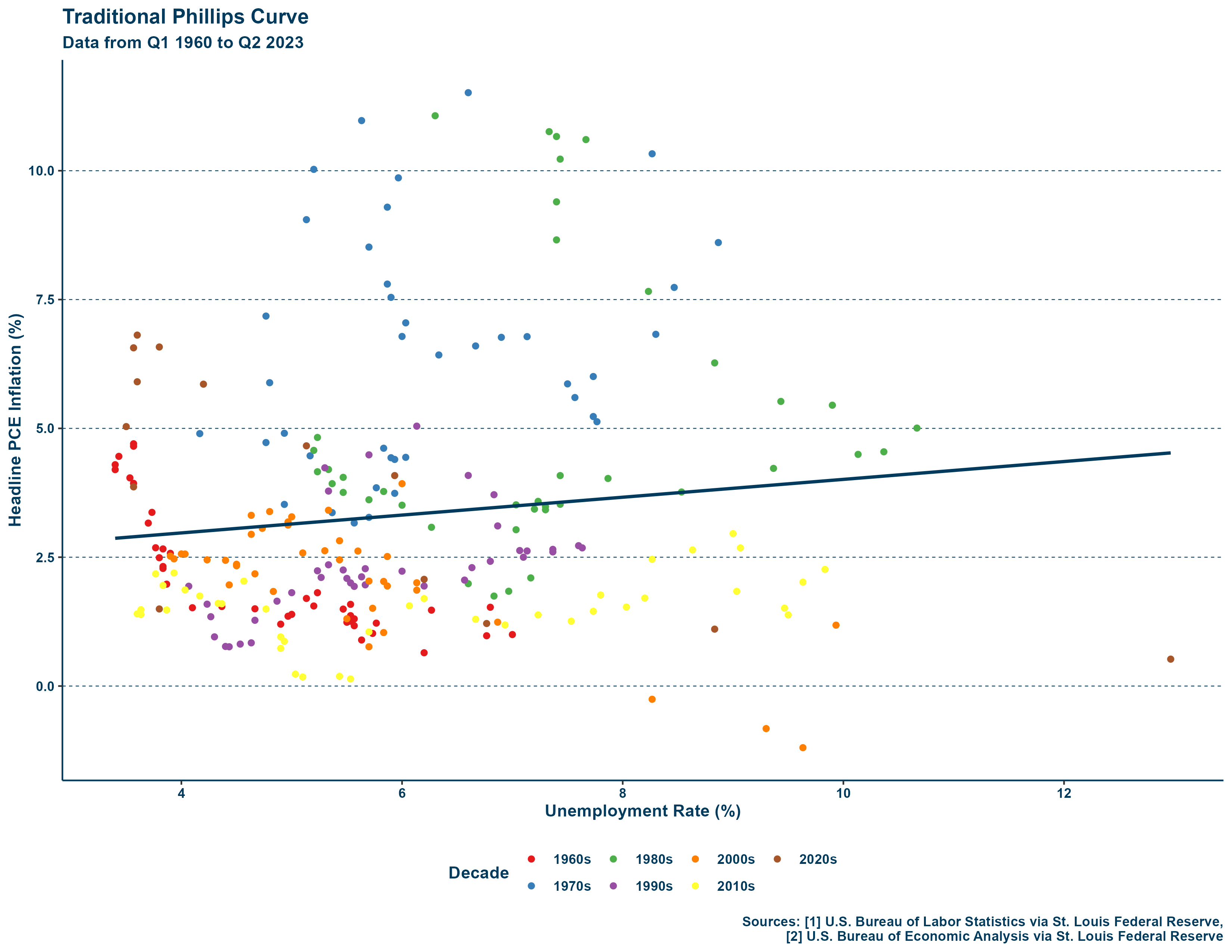
This representation demonstrates the central issue of the traditional curve—particularly in the 1970s—and why it is hardly even used anymore. I used data going back to the 1960s because it was available given that the traditional curve does not use the unemployment gap but rather the unemployment rate. As can be seen in the line of fit, the relationship between inflation and unemployment is not inverse over a period from the 1960s to the 2020s. If we were to zoom in on particular decades, we would see that the inverse relationship sometimes holds, but is completely upended in the 1970s—observable in seeing which decades most of the quarters of simultaneously high inflation and high unemployment are on the graph. The traditional curve is not up to the task and that is precisely why other specifications, like the accelerationist curve, have been more popular since the 1970s.
The accelerationist curve demonstrates the relationship between the change of the rate of inflation and the unemployment gap. Shown below is a graph with an accelerationist curve constructed by decade with the data from each quarter from Q4 1974 to Q2 2023:
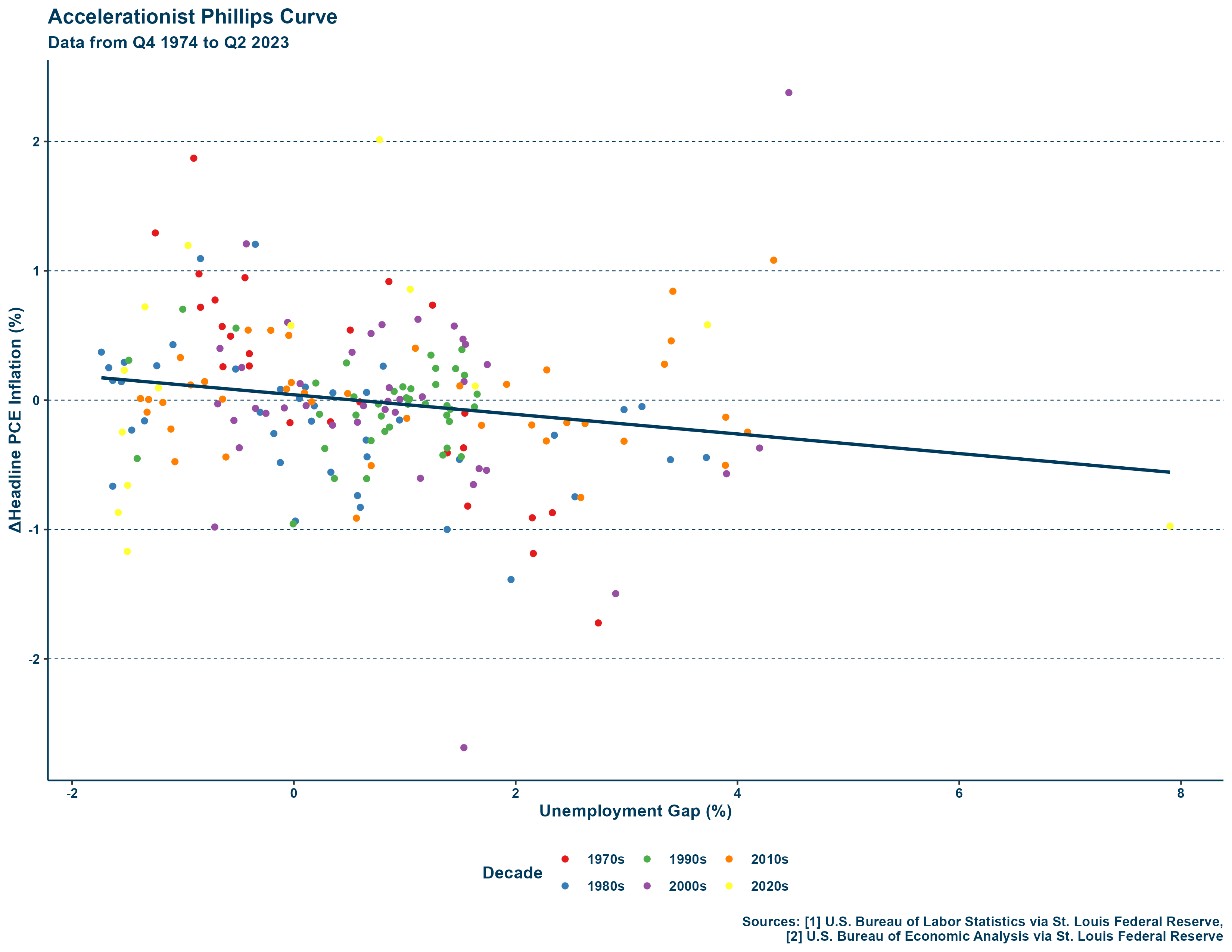
In contrast to the traditional curve, the accelerationist curve manages to maintain the inverse relationship over a period of decades. Does this mean that the accelerationist curve is a good specification? No, but it is at least a better one. To demonstrate why this alone is not sufficient, consider how the trend may look by decade. On the right is a graph of multiple accelerationist curves by decade, it is almost flat for several decades:
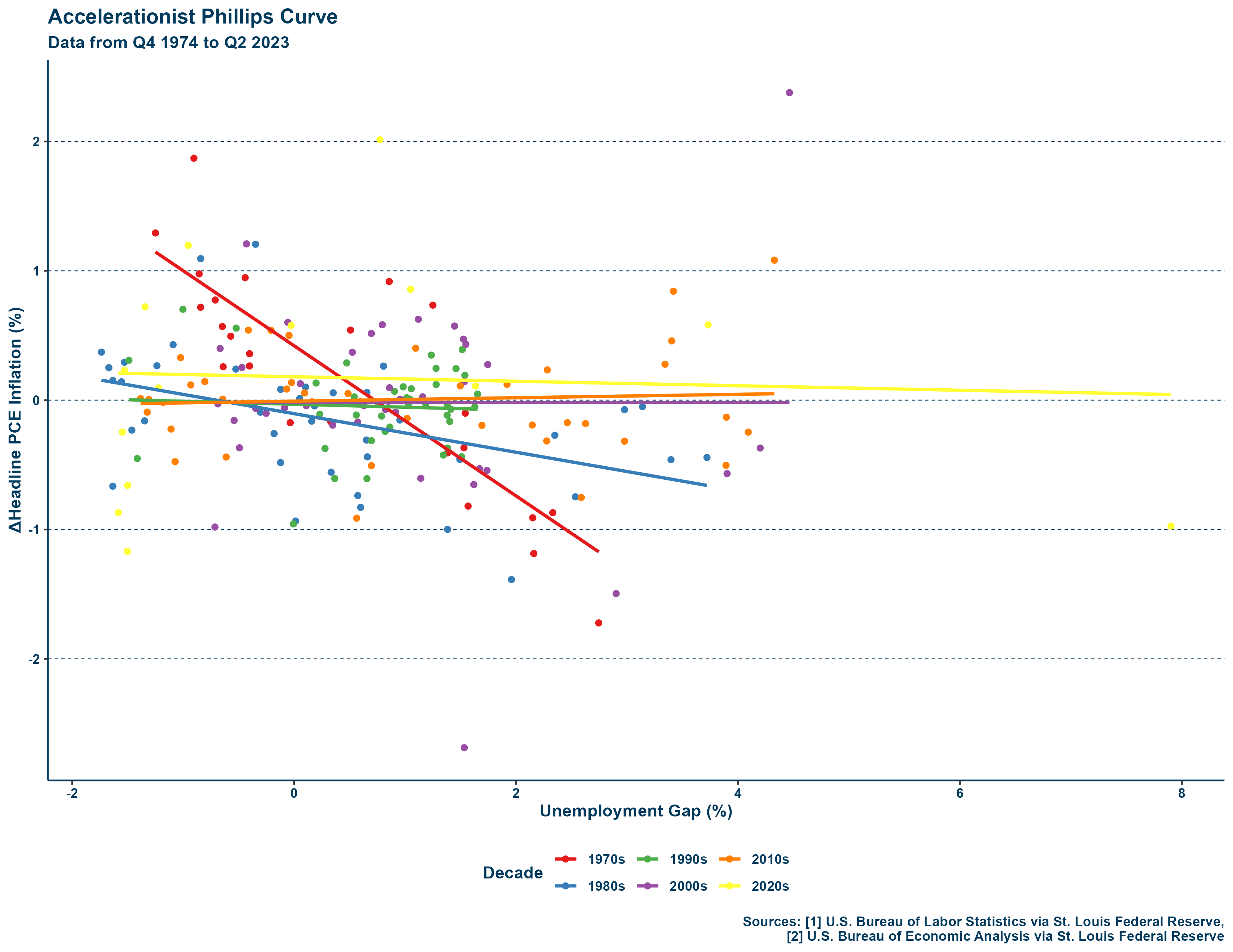
Although the accelerationist curve does do well with data from the 1970s many decades show an extremely slight inverse relationship (if at all), and the 2010s show a positive one! This is where the accelerationist curve fails. To go further, consider equation 5 from earlier. Running a regression of the unemployment gap on the change in inflation nets us the following:
This is not particularly bad, in fact since the actual changes in inflation swing more in both directions, the “aggregate” change within a given number of periods is not far off. The problem is that our \(R^{2}\) is small. A model including just the unemployment gap on the change in inflation accounts for a small percentage of variation in the change in inflation and that is clear in the graph above. To the right is the regression output using the “stargazer” package (Hlavac, 2020) for R:
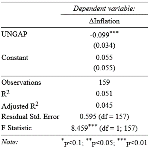
If one were to take the predicted values for the change in inflation from the estimation of this model for a period and the lagged inflation of preceeding period, they would get something that does not look terrible on first glance, but is quickly revealedd to be little more than a lagged chart of inflation give or take the tiny estimate for the change in inflation. Put another way, they would get something that looks like a slightly tweaked AR(1) model—not especially useful for actually modelling past (and particularly future) inflation.
The traditional curve is simply not suitable for showing its desired relationship between inflation and unemployment and the accelerationist curve does not make for a good model of it over time despite at least generally maintaining the expected relationship. With the varying failures of both perhaps there is truth in the death of the curve. Robert J. Gordon though, disagrees—the problem is not that the relationship is not there, you just need to through the kitchen sink at it—and so comes the triangle model.
5 The Mighty Trianlge (Model and Methodology)
The triangle model is not that radical of a change. It is like the accelerationist curve (recall how equation 5 is written) bar the fact that it includes supply shocks alongside the unemployment gap and lagged inflation (Gordon 2013). This single difference helps the model become far better at matching actual inflation with its predictions. The model used in this paper is adapted from the model used by Gordon (2013). Although that version was from a working paper, Gordon writes that the implementation is not far different from that of his 1997 paper. One significant difference between that implementation and that of this paper is the observation period. Gordon’s data (2013) goes from the 1960s to the 2010s whereas mine goes from the 1970s to the 2020s. For the Phillips curve to be dead, the relationship between inflation and unemployment would have to be a non-factor. As such, any results showing something contrary are signs of life. What matters though, is if the relationship can still be implemented such that a strong model of inflation can be constructed.
The model specified by Gordon includes the following: several lags of headline inflation (including moving averages), the unemployment gap and lags of it, the food energy effect (late period) and lags of it, the relative price of imports and lags of it, and the 8-quarter productivity trend and lags of it (Gordon 2013). I do not have data for the relative prices of imports, so the specification of the model used here is as follows:
\[ \pi_{t} = \beta_{0}+\beta_{1}MA\pi_{t-1}+\beta_{2}\pi_{t-2}+\beta_{3}\pi_{t-3}+\beta_{4}\pi_{t-4}+\beta_{5}MA\pi_{t-5} \] \[ +\beta_{6}\pi_{t-6}+\beta_{7}\pi_{t-7}+\beta_{8}\pi_{t-8}+\beta_{9}MA\pi_{t-9}+\beta_{10}\pi_{t-10} \] \[ +\beta_{11}\pi_{t-11}+\beta_{12}\pi_{t-12}+\beta_{13}MA\pi_{t-13}+\beta_{14}\pi_{t-14}+\beta_{15}\pi_{t-15} \] \[ +\beta_{16}\pi_{t-16}+\beta_{17}MA\pi_{t-17}+\beta_{18}\pi_{t-18}+\beta_{19}\pi_{t-19}+\beta_{20}\pi_{t-20} \] \[ +\beta_{21}MA\pi_{t-21}+\beta_{22}\pi_{t-22}+\beta_{23}\pi_{t-23}+\beta_{24}\pi_{t-24}+\beta_{25}(u_{t}-\overline{u_{t}}) \label{eq:model1} \tag{6} \] \[ +\beta_{26}(u_{t-1}-\overline{u_{t-1}})+\beta_{27}(u_{t-2}-\overline{u_{t-2}})+\beta_{28}(u_{t-3}-\overline{u_{t-3}})+\beta_{29}(u_{t-4}-\overline{u_{t-4}})+\beta_{30}fe_{t} \] \[ +\beta_{31}fe_{t-1}+\beta_{32}fe_{t-2}+\beta_{33}fe_{t-3}+\beta_{34}fe_{t-4}+\beta_{35}latefe_{t} \] \[ +\beta_{36}latefe_{t-1}+\beta_{37}latefe_{t-2}+\beta_{38}latefe_{t-3}+\beta_{39}latefe_{t-4}+\beta_{40}prodtrend_{t-1} \] \[ +\beta_{41}prodtrend_{t-2}+\beta_{42}prodtrend_{t-3}+\beta_{43}prodtrend_{t-4}+\beta_{44}prodtrend_{t-5} \]
The model itself clearly has some questionable aspects. For example, although inflation is only stationary at the 10% significance level (see below Augmented Dickey-Fuller test on Headline PCE), it is still not very kosher to use inflation rather than the change in it.
| statistic | p.value | parameter | alternative |
|---|---|---|---|
| -3.2027 | 0.089 | headline_inflation | stationary |
On the other hand, if this is good enough for Gordon, I struggle to believe that it could be completely wrong. This implementation can very fairly be described as throwing the kitchen sink at data. The thing is, that it also still does demonstrate the validity of the relationship first identified by Bill Phillips almost a century ago. After running the initial regression, I keep only the regressors that were significant (see appendix: “first_regression.png”), resulting in the final model:
\[ \pi_{t} = \beta_{0}+\beta_{1}MA\pi_{t-1}+\beta_{2}\pi_{t-4}+\beta_{3}MA\pi_{t-5}+\beta_{4}(u_{t}+\overline{u_{t}}) \] \[ +\beta_{5}fe_{t}+\beta_{6}fe_{t-1}+\beta_{7}latefe_{t}+\beta_{8}latefe_{t-1} \label{eq:model2} \tag{7} \]
Using a sample period covering Q4 1974 to Q2 2013 and equation 7, I estimate inflation from Q4 1974 to Q2 2023.
6 Results
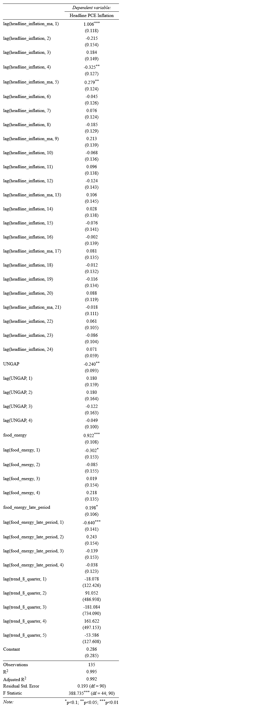
The results of the regression on the final model are included to the right:
Interestingly, the regression on the initial model did not find the second or third lag of inflation to be significant but did find the fourth lag to be. According to the regression results an increase in the contemporaneous unemployment gap is associated with a decrease in the inflation of a given period, so the relationship between the two holds strong and is still inverse! Interestingly, although an increase in the contemporaneous food energy effect is associated with an increase in inflation, an increase in the prior period is associated with a decrease in inflation. This appears to reflect a kind of “cooling” to inflation following spikes in food or energy prices in prior quarters. It is these latter kinds of effects that the triangle model captures, and the accelerationist curve does not is
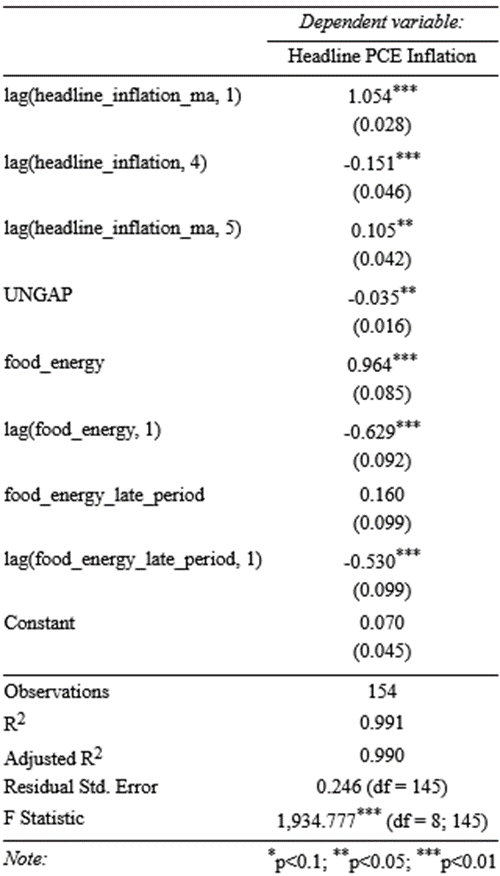
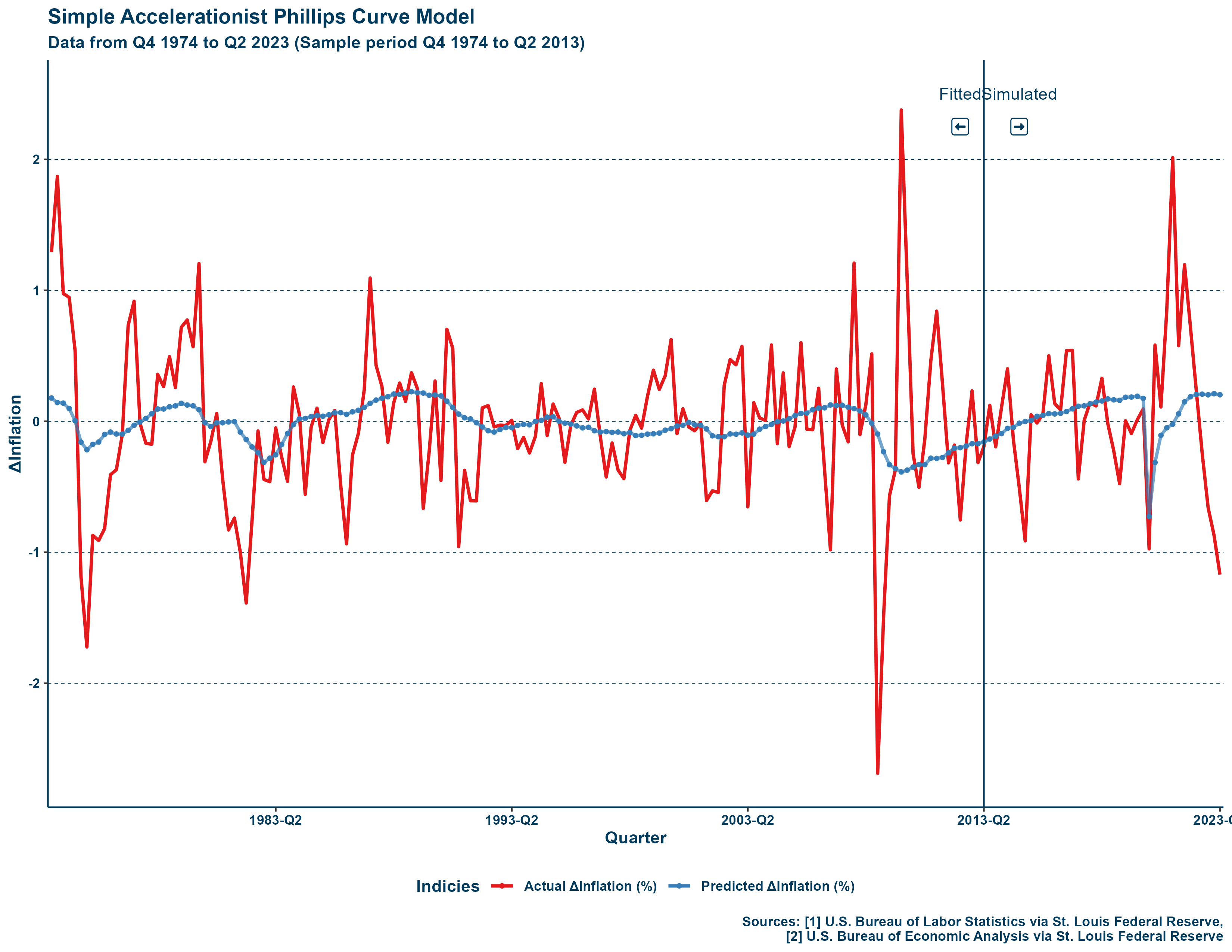
perhaps why the former serves as a better model of inflation overall. To illustrate this, I plot the estimates of the model, including those that are simulated (e.g., periods that were not included in the sample, Q2 2013 to Q2 2023), displayed below:
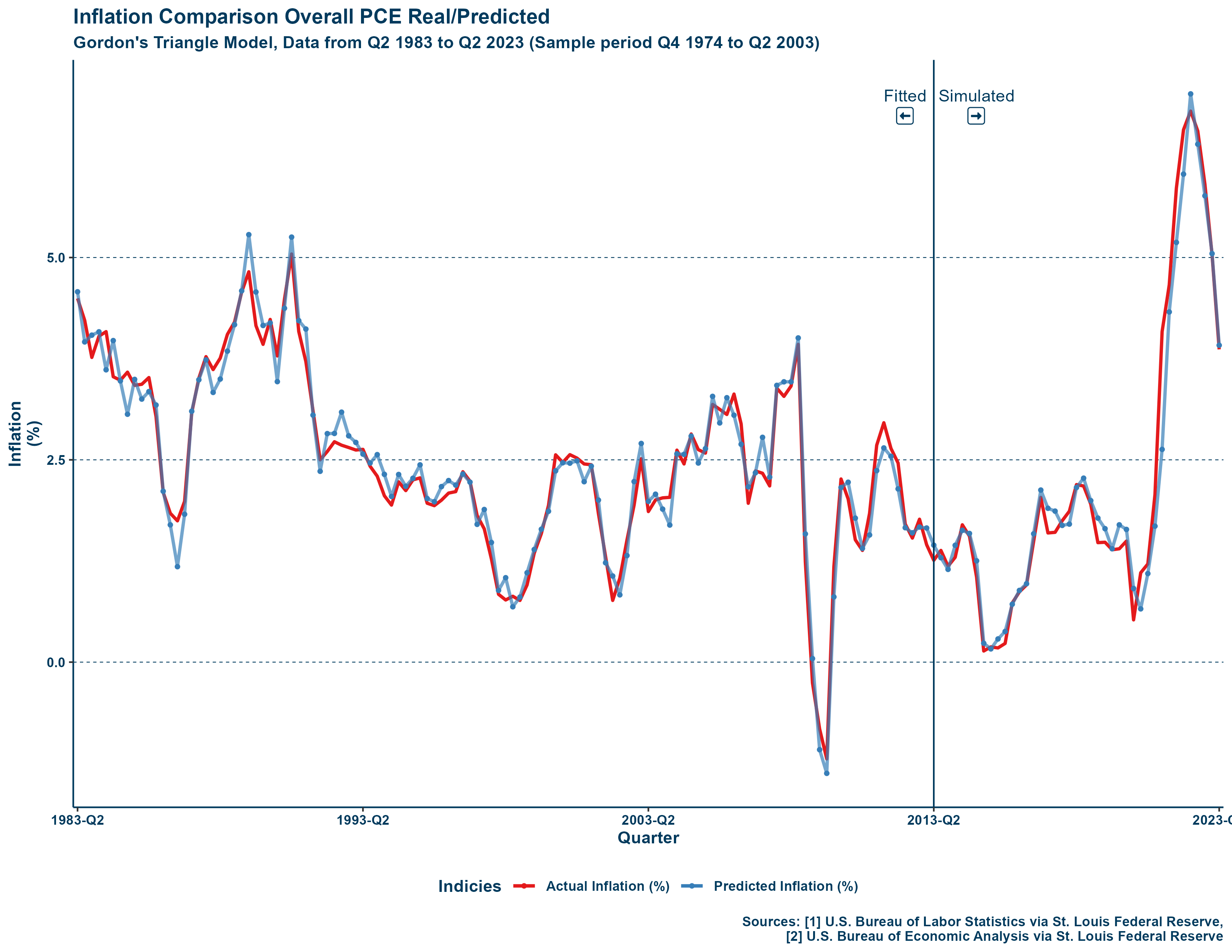
How could a dead curve be so accurate? While “eyeballing” is not the most advanced kind of statistical analysis, it is clear that the model does well at its purpose.
7 Conclusion
The Phillips curve is not dead, it is misspecified. Even without using short-run unemployment, which is better accoridng to Gordon (2013) for modern estimates, the triangle model provides accurate estimates for inflation, including for simulated periods. In his 1977 paper, Robert J. Gordon identified cost-push inflation, supply shocks, as a necessary component of any model trying to account for the stagflation of the 1970s and clearly he was on to something. Since then, he has updated his model every decade short of 2020. This is not a radical model, is it a better specification of a relationship identified 20 years earlier and it has been available for over half a century. To say the Phillips curve is dead is to ignore this and other attempts to better specify the relationship—consider even a non-linear curve or one based in conflict theory.
This paper took the triangle model as specified by Gordon (2013) and updated it with more recent data. The results of this paper are in alignment with those of the former, finding that the triangle model is a strong method for modelling inflation and that by extension, the relationship first identified in the traditional curve must still hold some value. The major findings of this paper are that the unemployment gap and food energy effect are still significantly related to the inflation rate a decade on.
The traditional curve is dead—long live the traditional curve—and the accelerationist curve is insufficient, but that does not mean that the relationship is not there or cannot still be considered in policy decisions. Instead, we just have to add in additional factors to account for supply shocks, as Gordon et al. (1977);Gordon (1981);Gordon (1997);Gordon (2013) does. Look no further than Jerome Powell’s attempts to increase unemployment to decrease inflation this very year. I doubt the Federal Reserve would be relying so much on a “dead” idea.
8 References
9 Appendix
DATA.R
MODEL.R
DataCleaned.csv
DataComplete.csv
GordonModelDataset.csv
First_regression.png