American Road Density

Tip🏡 Resume

1 Introduction

I have been wondering about how infrastructure reaches people. More specifically, I have been wondering about how it reaches people in different places. It is no shock to say that urban spaces are more developed in this sense than rural ones, the former simply have more stuff, but what if we could visualize that divide on a broader scale? Could we find a suitable stand-in for “infrastructure” in general, and then reference it in terms of the size of an area or the number of people it serves? Would we see a distinction between those measures? That is the theme that incited this short project, and I think there is a relatively easy stand-in found in the United States.

The United States is a car country; I doubt this statement needs much explanation or defense. As a car country, its infrastructure is defined by roads, so they should be as suitable a stand-in as any. The core idea for this project is thus to take data on American roads and counties, and use the lengths of roads as a stand-ins for infrastructure. We will then compare this measure across different aspects of county-level data (the area and population of each county) to asses/map how much different parts of the country are serviced (how much infrastructure they have). For our data, we use the tigris and usmap packages for road and county data respectively.

Presumably, we may expect that the proportion of roads to county area is higher among smaller counties, and we know that county sizes tend to be larger towards the Western half of this country (the United States), so we should see higher proportions in the East. Conversely, we know that the population of this country is largely concentrated in the East, so we may anticipate a higher proportion in the West, given that some areas there are extremely sparsely populated. Let’s see what we get.

2 Data and Code

Using total road lengths as a stand-in for American infrastructure, we aim to collect data on the road lengths of all roads across all counties in the United States. To get this data, we use the tigris roads() function, and supply FIPS county codes from usmap. We do this iteratively, since roads() works for only one FIPS code at a given time, and calculate the lengths of each road returned. We take our results and construct a new dataframe containing the respective FIPS code, LINEARID (a unique ID for a road in a given county), MTFCC (“MAF/TIGER Feature Class Code,” the class of road), and road lengths for each. We then take this new data and generate some statistics by referencing road lengths against the total areas and populations of each county. We use the most recent years available for this data from each source: 2024 for the roads and county geometries, and 2022 for the populations¹.

ImportantCode

# Road Density

# counties

counties_geoms <- us_map(regions = "counties", data_year = 2024)
counties <- as.data.frame(counties_geoms) %>% mutate(state = substr(fips, 1, 2), county = substr(fips, 3, 5))%>% select(state, county)

# roads()
# LINEARID is a unique ID for a road, but a road can be in more than 1 county
# Luckily, when a road is in a different county, the length in that county is
# recorded with a duplicated LINEARID rather than being added in the same entry.

for (i in 1:nrow(counties)) {
  roads_i <- roads(state = counties[i,1], county = counties[i,2], year = 2024) %>% 
    mutate(road_length = as.numeric(st_length(.))) %>% 
    as.data.frame() %>% select(-geometry)
  if(i == 1) {
    counties_roads <- data.frame(
      fips = paste0(counties[i,1], counties[i,2]),
      linearid = roads_i$LINEARID,
      mtfcc = roads_i$MTFCC,
      road_length = roads_i$road_length
    )
  } else {
    counties_roads <- rbind(
      counties_roads,
      data.frame(
        fips = paste0(counties[i,1], counties[i,2]),
        linearid = roads_i$LINEARID,
        mtfcc = roads_i$MTFCC,
        road_length = roads_i$road_length
      )
    )
  }
}
# write_csv(counties_roads, "counties_roads_list.csv")

# road stats
# use https://www2.census.gov/geo/pdfs/reference/mtfccs2022.pdf
# for reference to the types of roads
# counties_roads %>% select(mtfcc) %>% unique()

counties_roads_stats <- counties_roads %>% group_by(fips, mtfcc) %>%
  summarize(
    road_count = n(),
    road_length = sum(road_length, na.rm = FALSE)
  ) %>%
  left_join(counties_geoms %>% mutate(county_area = as.numeric(st_area(.))) %>% as.data.frame() %>% select(-geom), by = "fips") %>% 
  left_join(countypop %>% select(fips, pop_2022), by = "fips") %>% 
  mutate(
    road_count_to_county_area = road_count/county_area,
    road_length_to_county_area = road_length/county_area,
    road_count_to_county_pop = road_count/pop_2022,
    road_length_to_county_pop = road_length/pop_2022
  ) %>% ungroup() %>% rename(state_abbr = abbr, state_full = full) %>% 
  select(state_abbr, state_full, county, fips, county_area, pop_2022, mtfcc, 
  road_count, road_length, road_count_to_county_area, road_length_to_county_area,
  road_count_to_county_pop, road_length_to_county_pop)
# write_csv(counties_roads_stats, "road-density/counties_roads_stats.csv")

Our code above gives us a dataset that includes all MTFCC codes across each county, which means that we can filter down to specific classes of roads by county. Many of these classes aren’t for the roads we are thinking of, so we will focus on and filter for the following: S1100, S1200, and S1400, which reflect primary, secondary, and local roads as outlined in Table 1 below.

ImportantMTFCC Table

Table 1: Relevant MAF/TIGER Feature Class Codes Definitions

MTFCC	Feature Class	Description
S1100	Primary Road	Primary roads are limited-access highways that connect to other roads only at interchanges and not at at-grade intersections. This category includes Interstate highways, as well as all other highways with limited access (some of which are toll roads). Limited-access highways with only one lane in each direction, as well as those that are undivided, are also included under S1100.
S1200	Secondary Road	Secondary roads are main arteries that are not limited access, usually in the U.S. highway, state highway, or county highway systems. These roads have one or more lanes of traffic in each direction, may or may not be divided, and usually have at-grade intersections with many other roads and driveways. They often have both a local name and a route number.
S1400	Local Neighborhood Road, Rural Road, City Street	Generally a paved non-arterial street, road, or byway that usually has a single lane of traffic in each direction. Roads in this feature class may be privately or publicly maintained. Scenic park roads would be included in this feature class, as would (depending on the region of the country) some unpaved roads.
S1500	Vehicular Trail (4WD)	An unpaved dirt trail where a four-wheel drive vehicle is required. These vehicular trails are found almost exclusively in very rural areas. Minor, unpaved roads usable by ordinary cars and trucks belong in the S1400 category.
S1630	Ramp	A road that allows controlled access from adjacent roads onto a limited access highway, often in the form of a cloverleaf interchange.
S1640	Service Drive usually along a limited access highway	A road, usually paralleling a limited access highway, that provides access to structures along the highway. These roads can be named and may intersect with other roads.
S1710	Walkway/Pedestrian Trail	A path that is used for walking, being either too narrow for or legally restricted from vehicular traffic.
S1720	Stairway	A pedestrian passageway from one level to another by a series of steps.
S1730	Alley	A service road that does not generally have associated addressed structures and is usually unnamed. It is located at the rear of buildings and properties and is used for deliveries.
S1740	Private Road for service vehicles (logging, oil fields, ranches, etc.)	A road within private property that is privately maintained for service, extractive, or other purposes. These roads are often unnamed.
S1750	Internal U.S. Census Bureau use	Internal U.S. Census Bureau use.
S1780	Parking Lot Road	The main travel route for vehicles through a paved parking area. This may include unnamed roads through apartment/condominium/office complexes where pull-in parking spaces line the road.
S1810	Winter Trail	A type of seasonal trail, created and marked in snow, primarily traveled by snowmobiles and dog sleds, and used to reach housing units and to connect communities.
S1820	Bike Path or Trail	A path that is used for manual or small, motorized bicycles, being either too narrow for or legally restricted from vehicular traffic.
S1830	Bridle Path	A path that is used for horses, being either too narrow for or legally restricted from vehicular traffic.

3 Results

Having filtered down the road classes that we are concerned with, we create the following plots:

(a) Road Length v. County Area

(b) Road Length v. County Population

Figure 1: Road Length Charts

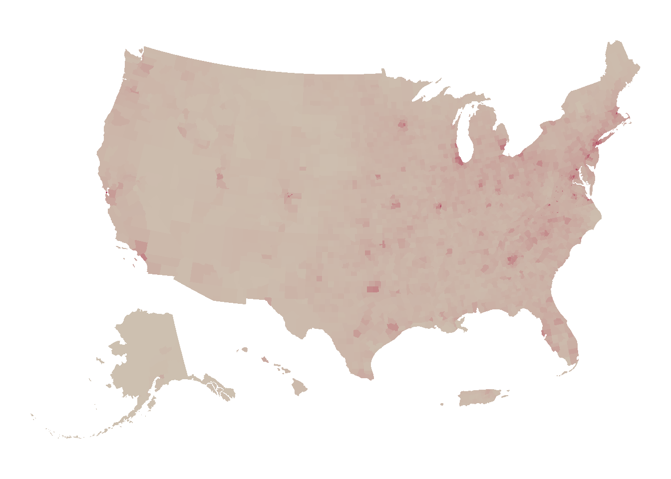
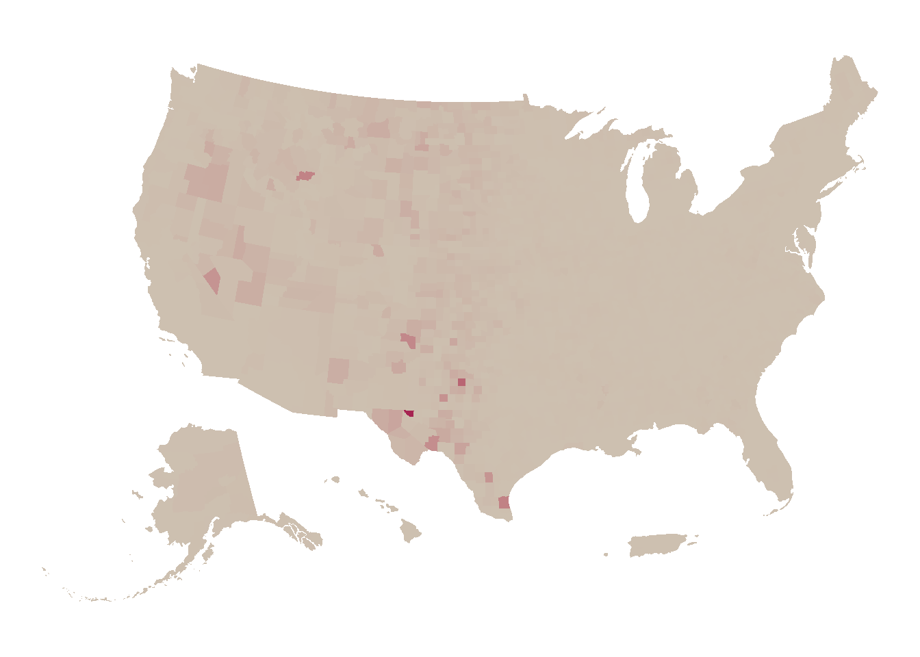
As we can see in the charts above, the proportions are in line with what we anticipated at the outset; the proportion of road length relative to county area is observably higher in the East than in the West, whereas the proportion of road length relative to county population is higher in parts of the West. Each chart shows relative ratios, and the scales are naturally different between them. What matters for our case is the visible magnitude, and we can see very clearly where the hot spots are in each map. The fact that Figure 1 (b) in particular is largely so blank tells us just how lopsided the relative ratio of roads to population is in the Western United States when compared to the East. From our charts, fewer people are served by relatively more “infrastructure” in parts of the West, whereas there is overall more infrastructure spanning smaller areas in the East. The data for this project is available here.

Footnotes

1. The distinction between 2022 and 2024 should not be especially large, but it is worth noting that the years are different.