| scenario | result |
|---|---|
| None Dropped | 79.91 |
| 10 Dropped | 85.90 |
Dropping Scores
1 Pondering Thy Grade Inflation
A friend of mine asked a question some time ago, the gist of it being: what is the optimal number of quizzes to drop, if you are a teacher/instructor/lecturer/professor (et cetera infinitum) in the business of dropping quizzes? Now, if the question is just about getting the highest scores, then the answer is pretty simple: give a bajillion quizzes and only keep the highest single result per student. That would obviously result in the highest class average, but it wouldn’t be very efficient, would it1? Similarly, assuming some normal distribution of scores by student, the improvement to scores per quiz dropped relative to a baseline of none dropped would just be the inverse of that distribution; e.g., a high return from the first and last quizzes dropped, and a low return from those around the mean (if dropping scores in order from lowest to highest \(n-1\) quizzes). This is because the first scores dropped would eliminate the lowest edge of the distribution, and thereafter the improvement from additional drops would be small until you remove enough to see a large return in aggregate. So, rather than considering scores relative to a case where none are dropped, what is the incremental improvement to scores per quizzes dropped relative to prior drops? Let’s think of an example:
You distribute 20 quizzes to each student in your class over the course of a semester. You drop the single lowest quiz, and see a large return to scores. Assuming a normal distribution of scores, how many more quizzes can you drop, before the improvement per total dropped, compared to the prior number dropped, flattens out? Keeping only the highest score per student returns higher average scores across students than keeping the two highest scores, but when you have already chopped 18 scores off (just about the whole of the distribution below the maximum), is the relative improvement to scores from dropping the second-highest very high? No; not unless the distribution is insanely skewed.
Thinking intuitively, the highest incremental improvements would come from the first drops, and thereafter the improvement should decline. This is because, as before, the first drops will be from the lowest end of the distribution, but, since we are looking incrementally, the “disaggregated” effect of each additional drop we don’t see such a large shared return from the high end of drops. To elaborate, if we were to add the gains from all increments from 0 v. 1 through 18 v. 19, it would likely come out as the same number as the gain from 0 v. 19; but 18 v. 19 will be much smaller than 0 v. 19.
Our aim, either way, is to see what number of scores are dropped where we get the most value out of our increments. Of course, assuming a normal distribution of scores, it should be pretty obvious that the most important score to drop in any case is the lowest one, because it will be very low (unless you set the minima to truncate at at a higher level); the truth is that this whole endeavor is an excuse to make something fun (skip to Section 3 for that). While different results will come from setting different minima/maxima/means, ever case there is arbitrary, and reliant on the scenario… so, I put together a little tool to set those things and illustrate a given case.
2 Math
Let’s get the first part out of the way. Assuming a (truncated) normal distribution of scores around a given mean, changing the number of quizzes given shouldn’t matter much in terms of the marginal improvement from the proportion of quizzes dropped. In other words, our marginally-efficient proportion of quizzes dropped should be applicable across any n number of quizzes distributed, assuming that the distributions are consistent and that each quiz is roughly centered around the same mean.2 Below is a function that takes the following:
n: the number, \(n\), quizzes distributed;dropCount: the number of quizzes dropped;mean: the mean result of each quiz;nLoop: the number of times that we loop our results to take averages among cases;nDrop: the number of quizzes remaining after the drop; andtrial_i: a vector containing the result of each loop.
to return the average score by student across \(n-n_\text{dropped}\) quizzes distributed with a given common mean for each quiz. The standard deviation used here is arbitrarily assigned as \(\frac{1}{10}\) of the given mean, and the limits to the distribution (beyond which values are truncated) are 0 and 100, respectively.
quizDropLoop <- function(n, dropCount, mean, nLoop){
  if(dropCount < n){
    nDrop <- n - dropCount
    trial_i <- c()
    for (i in 1:nLoop) {
      trial_i <- append(trial_i, mean(sort(rnormTrunc(n = n, mean = mean, sd = mean/10, min = 0, max = 100), decreasing = TRUE)[1:nDrop]))
    }
    return(trial_i)
  } else {
    print("uh oh")
  }
}
2.1 Example
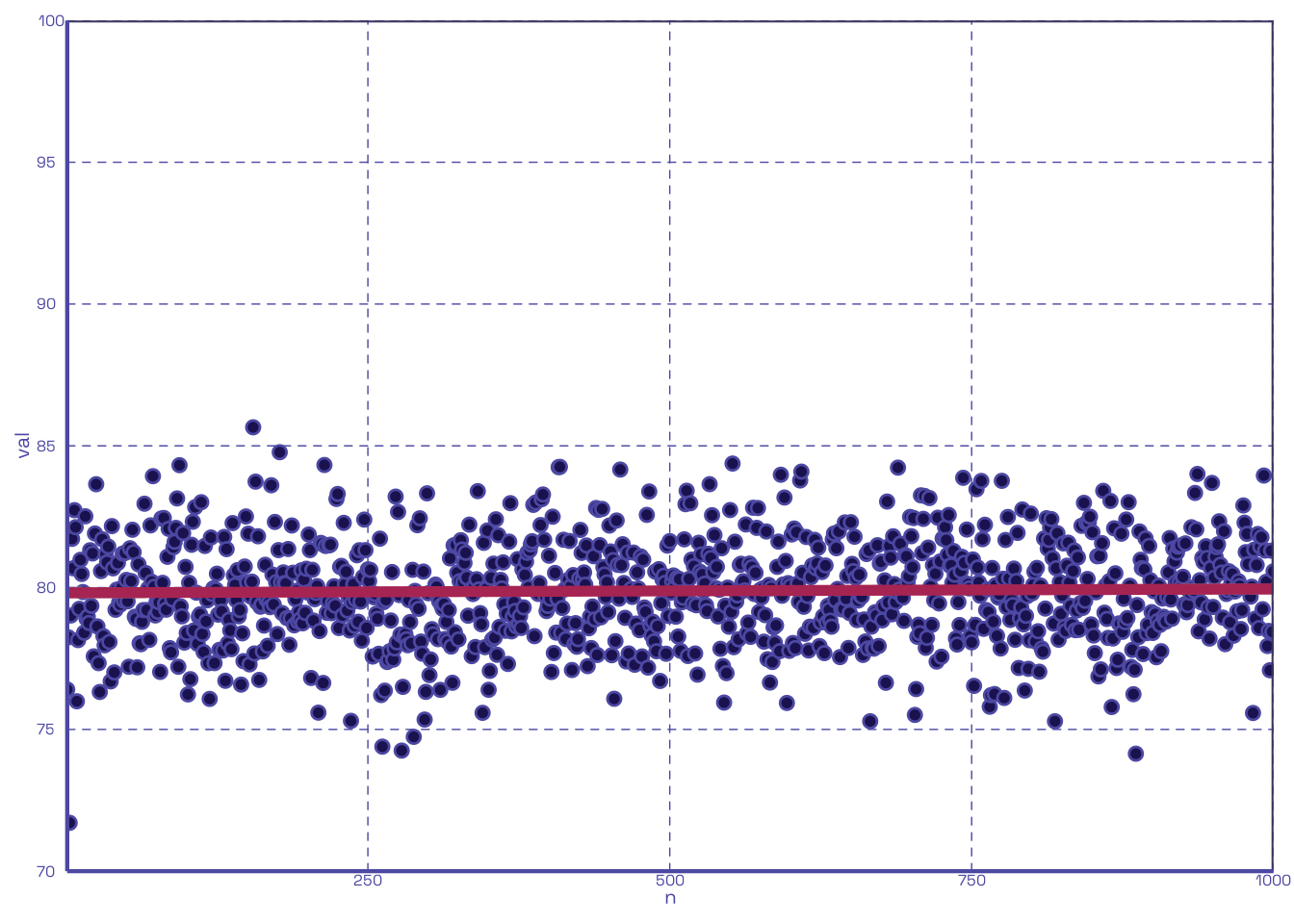
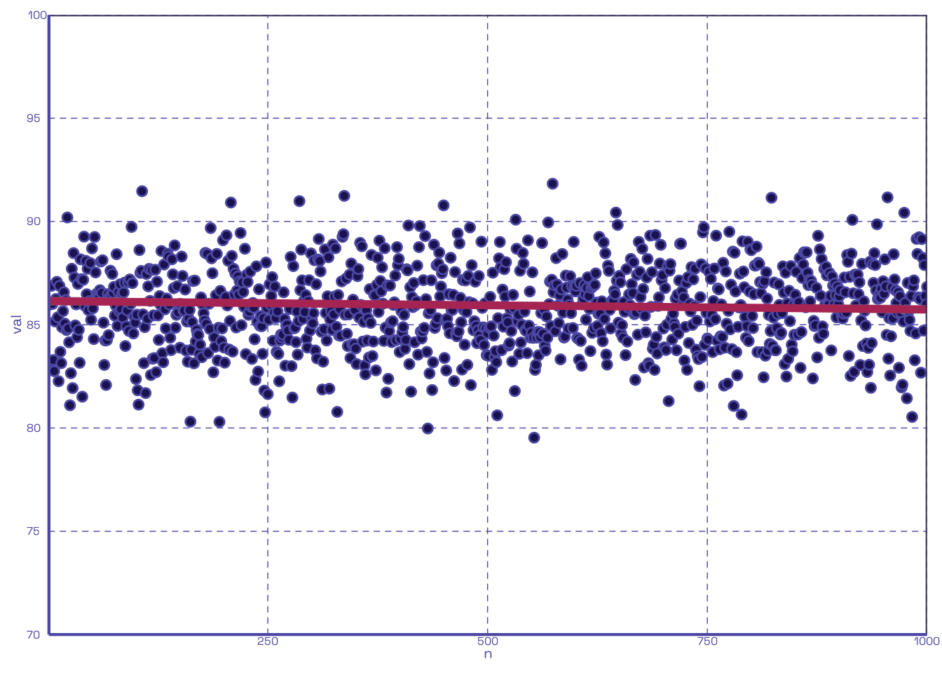
With this in-hand, let us assume a simple comparison scenario to test this function; 20 quizzes per student are distributed throughout the whole of the class curriculum3, with one scenario having 0 dropped, and the other having the lowest 10 each dropped. We will use 80 as our mean quiz score and we will take the mean of 1000 loops for each scenario:
Well look at that, dropping the lowest half of quizzes boosts the average; who’d’ve thought? We can also plot out the same two scenarios to show their respective clumps of scores:
2.2 The Fun
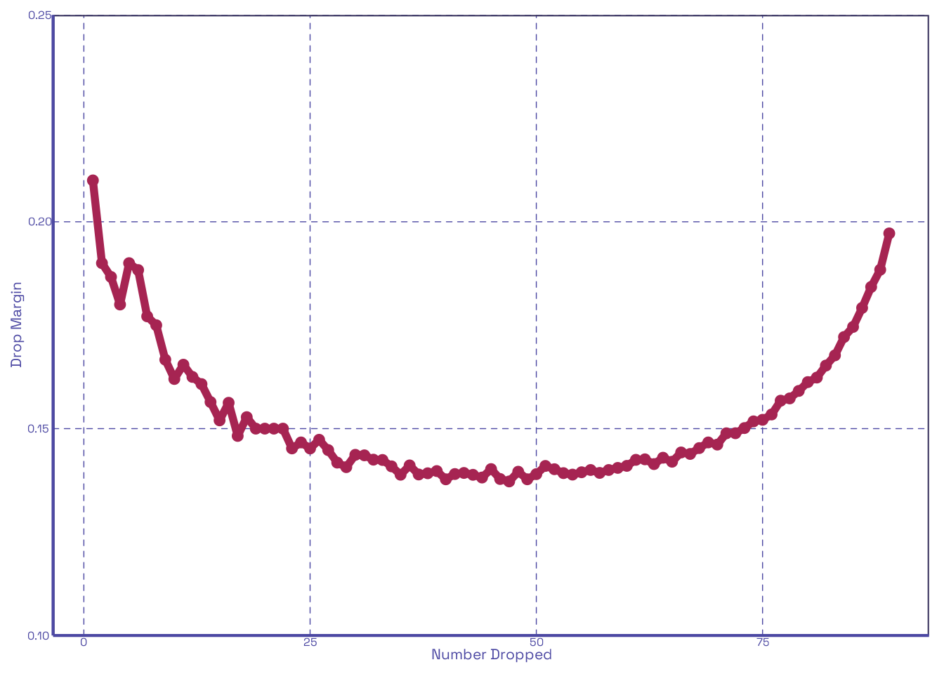
Let’s extend our prior scenario in Section 2.1 to cover a range of possible values for dropCount. Using the same number of quizzes distributed per student (20), the same mean (80), and the same number of loops (1000), but iterating dropCount from 1 through \(n-1\), let us calculate the improvement to scores relative to no drops and the improvement per each increment of drop:
| Number Dropped | Drop Margin | Incremental Margin |
|---|---|---|
| 1 | 0.8300000 | 0.7600000 |
| 2 | 0.7150000 | 0.3500000 |
| 3 | 0.6600000 | 0.2000000 |
| 4 | 0.6825000 | 0.1525000 |
| 5 | 0.6520000 | 0.1140000 |
| 6 | 0.6383333 | 0.1000000 |
| 7 | 0.6100000 | 0.0700000 |
| 8 | 0.6125000 | 0.0662500 |
| 9 | 0.6233333 | 0.0711111 |
| 10 | 0.6040000 | 0.0560000 |
| 11 | 0.6027273 | 0.0527273 |
| 12 | 0.6116667 | 0.0525000 |
| 13 | 0.6076923 | 0.0538462 |
| 14 | 0.6235714 | 0.0500000 |
| 15 | 0.6286667 | 0.0493333 |
| 16 | 0.6556250 | 0.0718750 |
| 17 | 0.6711765 | 0.0476471 |
| 18 | 0.6955556 | 0.0594444 |
| 19 | 0.7326316 | 0.0752632 |
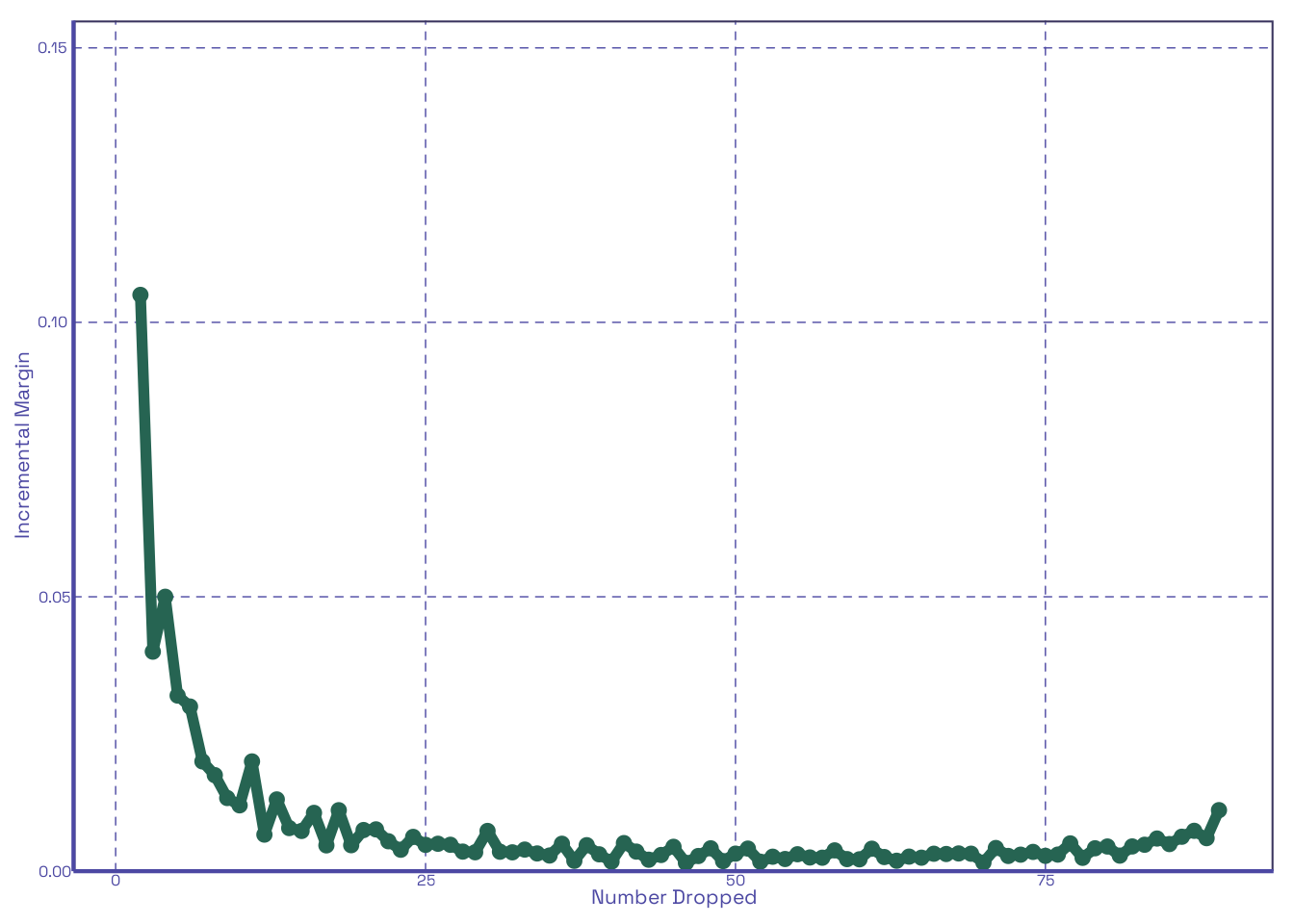
Table 2 shows us both the marginal improvement of a number of dropped quizzes relative to none being dropped, and the improvement by increment of quiz dropped. As noted in Section 1, the former just reflects the inverse of our given score distribution, whereas the latter begins high, and quickly flattens. We can see this clearly when plotted:
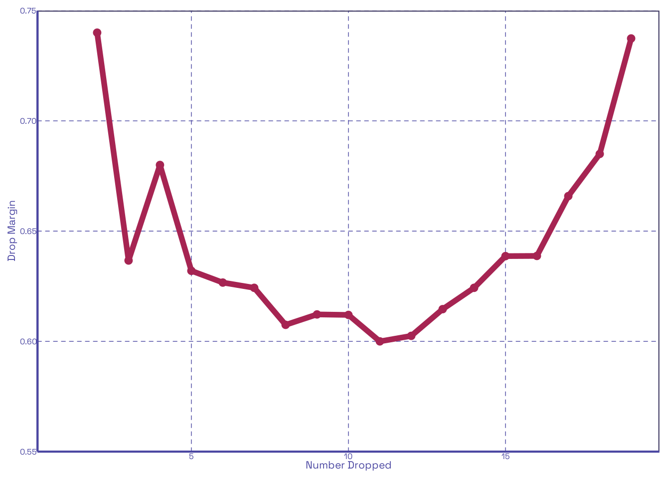
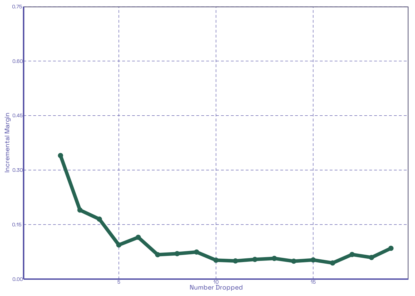
It looks like the first 2 to 3 drops in Figure 2 (b) have the largest effect on improving scores among the 20 quizzes distributed. Lets see how this changes if we change the number distributed; let’s say, 90:
In Figure 3 (b) the gap from the second to third drop widens enough that it’s clear that the first two are what really matter. This is entirely within expectations. With all this done, it’s pretty clear that our function does what we think it does. Now let’s make it interactive!
3 Interactive Dropper
For this part, we just modify our original function to allow user-input for the standard deviation, minimum, and maximum. We also limit the max number of trials to make things faster.
Footnotes
Won’t someone please think of the poor TAs having to grade 30 quizzes only for 29 to be dropped anyways.↩︎
Since we’re working with whole numbers (we’re not dropping half a quiz), there can be variation with the real number dropped across even v. odd cases, but on average this really should not matter much. The assumption about the means for each quiz has to do more with individual students than the quizzes; some students do not average the same as others, but let us assume that a given student with get roughly consistent scores across their quizzes, on average.↩︎
The “time” doesn’t really matter; it’s just all the quizzes ever given for that class.↩︎