Ready to Join?

Assessing the Effects of Joining the EU Through the Lens of the Phillips Curve

Author

Tin Skoric

Published

May 2025

Abstract

What does membership in the European Union entail for the states that sign on? In early 2020, for example, the United Kingdom left, and that move had serious implications for both British labor and prices—although they are muddied by the CoVid-19 pandemic. This known case of the effects of extit{leaving}, provides the useful base for the opposite: what happens to the join-ers? In this paper, I investigate the underlying shifts of the economies of those who extit{join} the European Union using panel data. I elect to focus on the 2004 enlargement, and implement a variation of Robert J. Gordon’s “Triangle” model of inflation considering a data period spanning from January 2001 to January 2007. I find that there was higher headline inflation, on average, among those who joined in the 2004 enlargement than among those who either did not or were already members. Otherwise, the model failed to find a traditional Phillips curve relationship present across groups of countries in the data.

🏡 Resume

1 Introduction

Approximately two decades ago¹, the European Union (EU hereafter) engaged in its most expansive enlargement to date. A total of ten nations ascended in May of 2004, many of which were, only two decades then-prior, Soviet satellite states. In short time, some of these same states have grown exceptionally, both since their independence, and since their ascension Among them, Poland saw growth that in some periods outpaced that of any other state in Europe—and has steadily transitioned from its status as a coal mine for the “Iron Curtain” to a new digital economy. One of the largest companies on the Warsaw Stock Exchange is “CD Projekt,” a video game company (“WIG20 INDEX Constituents” 2025). It is hard to describe the transformation of these states in such short order. However, a question arises when thinking about such cases. The growth we see in countries like this occurred over periods that include both their respective breaks from the Soviet bloc and their respective ascensions into the EU, so, what this paper studies is quite simple: how are the economies of states affected in particular by their ascensions to the EU? What does joining the EU do for you?

To study this question, this paper implements a variation of Robert J. Gordon’s “Triangle” model of inflation—itself an expansion of Bill Phillips’ traditional Phillips curve. This model is applied to a dataset comprised of groups of countries: those in the EU prior to the 2004 enlargement, those joining the EU in 2004, and those who did not join the EU (or at least, did not join during the time period covered). This dataset includes observations for inflation (total, energy, and food) and unemployment collected over a period spanning from January 2001 to January 2007. More details on the model and methodology are included in the sections that follow (Section 2, Section 3, and Section 4). To rephrase the question in the context of the “Triangle” model, with a specific set of points to study:

Does the traditional Phillips relationship (inflation v. unemployment) hold, at least for our countries of interest, when implemented as a component of the “Triangle” model? There has been much talk of the curve being “dead” (Robert J. Gordon wrote his 2013 working paper, Gordon (2013), expressly intending to refute that point in the case of the United States), so it is worth seeing how it holds in general; and
Does the ascension of a state into the EU change that relationship? How so does that relationship change? More specifically, we would expect the relationship to be present, at least wheresoever it is present in general, and hopefully that it becomes more acute among “join-ers.”

The latter is not dependent on the former, and we need not worry if neither comes back as we would wish. In our many variations of the model, we do not find strong evidence to back the first part of the question, and the second only gets any “support” in terms of our expectations when we consider country-level fixed effects in the appendix extension, Section 7.1. We fail to find much evidence that there is a relationship, or that the relationship changes in the ways we would expect. Rather, it appears that the join-ers experienced higher levels of inflation, which contrasts with the direct bilateral comparison by Gylfason and Hochreiter (2022) (discussed in Section 2). It is quite probable that this would have happened had we been able to calculate the time-varying unemployment gap, but it is possible too that that alone accounts for much of our woes. Disappointing, but it is not for naught, and the process of this work illustrates well the challenges of applying old ideas to newer data. Before continuing, it is worth exploring a brief history of these modern economies and the EU as a whole. I think it important to demonstrate that the “Union” is not a particularly unified entity by illustrating how much more united Europe was dreamed to be in the post-war world. If nothing else, knowing where many of these states “came from” can help motivate us to understand why the question asked is of such value, and perhaps why our expectations should be tempered when thinking about models studying “Europe.”

1.1 The Political Economies of Post-War Europe

Approximately eight decades ago, British Conservative Party Prime Minister Winston Churchill—a man who had, among some admittedly less savory things, boldly steered his nation through the harsh and unforgiving tides of war—was ousted, by Labor Party leader Clement Attlee, in a landslide. This is one of the most stunning losses for the Conservative Party in the history of British parliamentary democracy—the British electorate wanted reform, and they voted for it. It was during the Attlee government, for instance, that the National Health Service (NHS), the national public healthcare system still in effect today, was established. Europe in the early post-war days was marked broadly by both a need to rebuild (Meurs et al. 2018b) and rising political aspirations to rebuild anew.

A key component of these aspirations, was a wave of “internationalism” calling for cross-state peace and cooperation. This was not a phenomenon unique to post-war Europe following the Second World War, but a rather common occurrence—Count Claude-Henri de Rouvroy of Saint-Simon had drawn up an idea for a united Europe “[…] on the eve of the Congress of Vienna” (Meurs et al. 2018b). What is notable, is that this was a wave of particularly acute strength. Per Meurs et al. (2018b):

In the early post-war years, ideas about federalist cooperation and strengthening the community of European states existed alongside even more ambitious prospects, such as so-called ‘world federalism’ […] To their [European federalists’] mind, the power of the nation states had to be broken. That process would politically integrate post-war Germany (the anticipated economic engine of Western Europe) without it having to be curtailed economically for fear of renewed German military aggression.

Although the notion of “world federalism” was ossified by the encroaching Cold War status quo, the European-level cause was bolstered in Western (and partly, Central) Europe, by fears of Soviet aggression. Moreover, there remained the strong economic incentives to rebuild via integration. Per Meurs et al. (2018b) once more:

After the war, the economies of European countries had to be rebuild [sic] once again. Just as in the 1930s, economies in Western European countries were heavily closed off to one another as a result of tariff barriers and other national protectionist measures. An even more urgent foreign trade problem for Western European countries was a shortage of dollars, caused by an increased demand for imports from America after the elimination of Germany as a capital goods supplier. This hindered exports for the United States. The government of the United States was willing to help, but insisted on European economic integration, a precondition for efficiency in production and, therefore, rising prosperity. Last, but not least, integration would facilitate American exports to Europe.

There was both a spirit—a plea—for peace on human grounds, and an economic need for cooperation post-war.

1.2 The European Union

Approximately seven decades ago, those post-war aspirations in Western (and Central) Europe were channeled into the reformation of the Anglo-French alliance into the “Western European Union” with an update to the Brussels Treaty (“BRUSSELS TREATY” 1994), which was itself soon thereafter joined by a series of “European Communities.” The former treaty was largely to do with military defense, but spares no time indulging readers in lovely internationalist rhetoric².

Yet, by the time of the latter—by the time the European Communities were being established—the rosiest of this language had already waned. The federalist dream was surely done-in by the simple reality that nation states valued their autonomy, and even functionalism (“[…] a method to effect unity in a stealthy manner” via technocratic “sectoral integration” (Meurs et al. 2018b)) was bleeding. The common market was there—in the Communities—but little else. In truth, the European integrative project was already less of a cohesive bloc than the early dreams. Rather, what was left was a move to expand the functions of their existing economic cooperation (Meurs et al. 2018a):

The ECSC [European Coal and Steel Community] and the Treaties of Rome marked both a farewell to ambitions of idealistic Europeanism that had encompassed the Council of Europe, and the rise of a functionalistic, technocratic Europe. The Treaty of Maastricht was the definitive breakthrough to a ‘political’ Europe. For a long time the European Community had limited itself to its common market. The Treaty of Maastricht introduced new policy areas, such as the founding elements for a common currency, a domestic policy and a foreign and security policy […] the most important European leaders were deeply aware of the necessity of further cooperation in these years.

In other words, the core economic incentives for cooperation still rang loud, but the speed with which dreams of “world federalism” devolved into the above-described resolution, should be telling of just how consistently-applied things are within the EU. To summarize: do not mistake “Union” to mean that all states derive even stakes. Some states, for example, receive block grants for development of infrastructure funded by other states. The states who today receive such grants (our friend Poland among them) may one day be issuing them—in which case, the economic effects that we observe may be quite different.

2 Literature Review

This paper applies a variation of Robert J. Gordon’s “Triangle” model to the question of how state-economies are affected by their ascensions to the EU. These two threads, in particular, have scarcely been paired together, so this section is split into three sub-sections, largely describing:

Works studying the economies of EU join-ers against those not;
Background on the Phillips curve provided by Phillips (1958); and
Works by Robert J. Gordon detailing the development of his model.

2.1 Prior Studies Concerning European Union Admission

This section will detail works Gylfason and Hochreiter (2022) by economists Thorvaldur Gylfason and Eduard Hochreiter, who have together penned a series of articles comparing post-Soviet (and/or post-Yugoslav) states who joined, or did not join, the EU. In their 2009 article (Gylfason and Hochreiter 2009), published in the European Journal of Political Economy, Gylfason and Hochreiter compare the development of two states: Estonia and Georgia. Both post-Soviet states, the latter has not joined the EU and was caught in a brutal civil war in its early years (1991 to 1993), while the former joined in 2004. The authors observe the divergences between the states through time (up to the year 2006), by applying a constant-returns-to-scale growth accounting model, and by directly contrasting macroeconomic datapoints among the two. In particular, Gylfason and Hochreiter stress the political-economic development of Estonia, compared to Georgia, in the form of the “EU perspective,” or as they (Gylfason and Hochreiter 2009) aptly summarize in their introduction:

We believe that the prospect of rapid EU integration, “the EU perspective,” provided a critical anchor for sustained political, institutional, and economic reforms across the political spectrum.

Within less than 15 years, Estonia was able to accede to the EU and its gross national income (GNI) per capita rose to a half of that of Finland […]

In contrast, Georgia, after regaining independence, was torn by civil war […] Georgia was caught in a low-income trap, and suffered from corruption as well as from weak economic and institutional reforms. The absence of an EU perspective in Georgia as well as of a calm relationship with Russia did not help.

In this work, the authors conclude that a core aspect of the successful development of these (post-Soviet) EU join-ers—or at least, Estonia—is the set of institutional reforms (political, economic, etc.) implemented as part of the ascension process, which pay dividends in the long-term, alongside the benefits of membership itself. Beginning as a relatively poorer state, Estonia has out-paced Georgia because of its reforms. Trade liberalization, competition, and getting inflation under control—these are the things Estonia did on its journey towards EU membership that Georgia has not seen nearly as much success in (Gylfason and Hochreiter 2009).

In their 2022 article (Gylfason and Hochreiter 2022), published in the journal of Comparative Economic Studies, authors Gylfason and Hochreiter continue with the bilateral comparisons to another post-Soviet pairing: Belarus and Lithuania. The former was (and is) a state that has not joined the EU, and remains deeply politically tied to the Russian Federation³. The latter, is a post-Soviet republic that—like Estonia—joined the EU in 2004. The authors similarly compare the two states directly, again using a “simple growth accounting model” (Gylfason and Hochreiter 2022)—observing outcomes—but do so over a longer time-frame (up to 2020) and observing conditions in terms of trade-offs. Specifically, Gylfason and Hochreiter find that the types of institutional reforms implemented in Lithuania as part of ascension (as like those implemented in Estonia), saw lower inflation (getting inflation under control) as being complemented by higher unemployment when compared to Belarus. It is lovely to imagine some kind of Phillips curve is in here somewhere⁴, but the authors resolve to largely confirm their findings from their 2009 paper (Gylfason and Hochreiter 2009).

In summary, across their works comparing post-Soviet states, authors Gylfason and Hochreiter find, indeed, that joining the EU, and the process of joining, and the associated institutional reforms, contribute greatly to the differential in growth between states that join and states that do not. Getting into the EU, is a path to growth for states⁵, even if—per Section 1.2—we understand that such gains may not be evenly distributed long term. The knowledge that institutional reforms on the road to EU membership are a component of the economic differential however, is something that we will have to reckon with in our own analysis. Additionally, these concern differences among countries who join and do not, whereas we are looking, largely (see: @sec-did in the appendix for something a little different), at differences between countries before and after joining.

2.2 The Fisher Phillips Curve

The “Phillips curve” (Phillips 1958) describes the inverse relationship between labor (typically and most traditionally via the rate of unemployment) and prices (typically via inflation, and, in the case of Bill Phillips specifically, wage price inflation). The work of Bill Phillips was not entirely novel⁶, but it took his name and as such this paper will continue to refer to the associated relationship as such.For a time, macroeconomic policy was considerably informed by this simply-identified curve—the New Dealers made good use of it and, to the best they could know, it proved useful. It is this very relationship that this paper makes use of to identify the changes among European economies joining the EU.

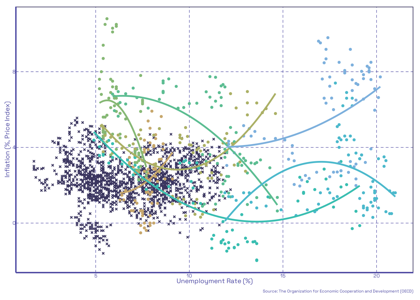
However, in the the curve was to be beset by its greatest foe, stagflation, in the 1970s, and in that era proved to not be a true rule. In fact, even looking at our own data (which will be further introduced in Section 3), it is clear that the traditional relationship (which, again, assets an inverse slope) just does not hold much across countries—at least our dataset of countries. For example, below is a plot of the Phillips relationship through time for our countries of most interest (the 2004 join-ers):

As seen in the above plot, there are only a few cases where the traditional relationship of interest is at all arguable. It is behind this backdrop that various “tweaks” to the Phillips curve would arise in hopes of making it work again. Among these, we attempts to consider changes rather than comparing variables that were arguably stationary processes. But, another idea arose, from the corner of Robert J. Gordon, the “Triangle” model of inflation⁷.

2.3 Gordon’s Triangle

Robert J. Gordon’s “Triangle” model of inflation Gordon (2013) was devised to address the weaknesses of other “tweaks” to the old Phillips Curve relationship. The model did this by incorporating additional variables, where Gordon defined headline (aggregate) inflation to be dependent on three underlying relationships:

“Underlying” inflation, accounting for predominant existing trends, or “inertia,” and functionally implemented as the lagged rate of inflation;
“Demand-pull” inflation, accounting for the traditional Phillips curve dynamic of labor v. prices, and functionally implemented in a variety of ways across Gordon’s works; and
“Cost-push” inflation, accounting for price shocks across specific segments of the economy that would result in shocks to the aggregate rate of inflation, and functionally implemented by including the rates of inflation for food, energy, and sometimes rental housing, and/or others.

In his later works, particularly his 2013 NBER (National Bureau of Economic Research) working paper, Gordon uses a time-varying unemployment gap derived by first calculating a time-varying natural rate of unemployment and taking the difference against the rate of unemployment Gordon (2013), much in the same way as Staiger, Stock, and Watson (1997). This is done to account for how the labor market may exercise non-constant influence across different times (and for us, different economies). Specifically, the time-varying rate of natural unemployment is derived from a cubic spline regression of a set of lags of unemployment on the core rate of inflation. From this, the intercepts are taken and divided by period (and in our case, state) to devise the rate. Then, this is subtracted from the unemployment rate by period and state to derive the time-varying unemployment gap. This gap allows implementations that include it to more thoroughly reflect labor trends and their effects given the conditions of their observation. As demonstrated in Gordon (2013), the unemployment gap tends to show coefficients of notably greater magnitude than those on the unemployment rate. Unfortunately, for this paper, the calculation of the time-varying natural rate proved extremely troublesome, and so the plain rate of unemployment is utilized for our implementation. This is a flaw, and it is hard to know how much this may have hurt our model.

Gordon is quick to note the achievements of the model, “[…] the model explained in advance in 1982 why the inflation rate fell so rapidly during 1981-86” (Gordon 2013), and while it is by no means a model grounded in modern methods to identify causal relationships⁸, it is a relatively simple (conceptually) and effective model for simulating inflation that still keeps the Phillips curve relationship at its core, and will thus be modified for our purposes.

2.4 This Contribution

Taking the prior works considering the differentials in outcomes between join-ers and non-join-ers, and applying a modified version of the “Triangle” model, this paper does something unique. The aim of this paper is to test both the continued (hint: not) strength of the Phillips curve, and to see how it applies in changes to economic dynamics among EU join-ers. For example, if Lithuania saw higher unemployment in exchange for lower inflation as per Gylfason and Hochreiter (2022), then a “spiritually” similar result would be to see a Phillips relationship at least among our join-ers, and hopefully one that notably changes in magnitude upon ascension in favor of the traditional inverse dynamic. Our contribution is this investigation.

3 Data

3.1 Collection

Data is collected from the Organization for Economic Cooperation and Development on inflation (total, food, and energy) and unemployment on the countries of interest (Hungary, Poland, the Slovak Republic, Latvia, Estonia, Lithuania, and Czechia), alongside many EU (European Union) member states (members prior to 2004)—and a few other non-EU countries such as the United States (but not ones that are otherwise in an EU trade bloc). We, unfortunately, do not include Slovenia in our final dataset, as there are insufficient observations for our purposes. We collect this data over a period of January 1990 through December 2007—although we restrict ourselves to only a subset of this (01/2001 to 01/2007) for analysis. We use only a subset, not just because some countries (including some countries of interest!) do not have observations for the 1990s, but because a number of the variables we generate for the purposes of the model require imposing lags (as will be discussed in Section 3.2), which puts additional constraints. We remain with 27 countries included in our final dataset—with 73 observations per county, totaling 1,971 observations across countries and through time. The source-datasets are available below as direct links:

Inflation Rate (percent, national—not Harmonized—CPI), Monthly. Includes: Total, Food (non-alcoholic drinks), and Energy. Not seasonally adjusted

Link: OECD, (DSD_PRICES@DF_PRICES_ALL) Consumer price indices (CPIs, HICPs), COICOP 1999
Unemployment (Among Persons Aged 15 and Older), Monthly. Includes: Total (in thousands) and Rate (in percent). Not seasonally adjusted.

Link: OECD, (DSD_LFS@DF_IALFS_INDIC) Infra-annual labor statistics

3.2 Shaping and Summarizing

From the sourced datasets, we select our necessary data and group it into a cleaned dataset. We also generate new lagged variables for the purposes of the model (see: Section 4). The variables in our completed dataset, including those generated, are listed and described in Table 1 below:

Table 1: Dataset Variables

Name	Description
PERIOD, $t$	The time period of the observation; year and month (YYYY-mm-dd format).
REF_AREA_ABBR, $i$	The three-letter abbreviated name of the country of the observation.
REF_AREA	The name of the country of the observation.
INF_ENERGY, $π^{e}$	Energy price inflation observation for the country and period.
INF_FOOD, $π^{f}$	Food price inflation observation for the country and period.
INF_TOTAL, $π$	Total inflation observation for the country and period.
INF_TOTAL_CHANGE, $Δ π = π_{t} - π_{t - 1}$	First-difference change in INF_TOTAL observation for the country and period.
INF_TOTAL_ROLLMEAN, $M A^{π} = \frac{1}{12} \sum_{t = T - 11}^{T} π_{t}$	12-Month rolling average of INF_TOTAL observations for the country and period.
INF_CORE, $π^{*}$	INF_TOTAL less INF_ENERGY and INF_FOOD observations for the country and period.
UNEMP_LEVL	Unemployment level observation for the country and period.
UNEMP_PERC, $u$	Unemployment percent observation for the country and period.
UNEMP_PERC_CHANGE, $Δ u$	First-difference change in UNEMP_PERC observation for the country and period.

Not all of the above variables are integral, or used, in the model, but all that remain are relevant and are either descriptively useful or otherwise worth retaining. Below is a table of summary statistics⁹ for variables that are used in the model(s):

Table 2: Summary Statistics (n = 1971)

Variable	Stats	Freqs. (% of Valid)
INF_ENERGY [numeric]	Mean (sd): 5.3 (6.2) min < med < max: -16.8 < 4.9 < 43.8 IQR(CV): 8.6 (1.2)	1956 distinct values
INF_FOOD [numeric]	Mean (sd): 2.5 (3) min < med < max: -7.3 < 2.1 < 18.5 IQR(CV): 3.7 (1.2)	1859 distinct values
INF_TOTAL [numeric]	Mean (sd): 2.6 (1.7) min < med < max: -2 < 2.4 < 10.8 IQR(CV): 1.8 (0.7)	1723 distinct values
UNEMP_PERC [numeric]	Mean (sd): 8.1 (3.8) min < med < max: 1.7 < 7.6 < 21 IQR(CV): 4.4 (0.5)	239 distinct values
pre2004member [integer]	Min: 0 Mean: 0.6 Max: 1	0: 876 (44.4%) 1: 1095 (55.6%)
inEU2004 [integer]	Min: 0 Mean: 0.7 Max: 1	0: 645 (32.7%) 1: 1326 (67.3%)
INF_TOTAL _ROLLMEAN [numeric]	Mean (sd): 2.6 (0.6) min < med < max: 1.1 < 2.5 < 4.5 IQR(CV): 0.7 (0.2)	1971 distinct values

INF_ENERGY

[numeric]

Mean (sd): 5.3 (6.2)

min < med < max: -16.8 < 4.9 < 43.8

IQR(CV): 8.6 (1.2)

1956 distinct values

INF_FOOD

[numeric]

Mean (sd): 2.5 (3)

min < med < max: -7.3 < 2.1 < 18.5

IQR(CV): 3.7 (1.2)

1859 distinct values

INF_TOTAL

[numeric]

Mean (sd): 2.6 (1.7)

min < med < max: -2 < 2.4 < 10.8

IQR(CV): 1.8 (0.7)

1723 distinct values

UNEMP_PERC

[numeric]

Mean (sd): 8.1 (3.8)

min < med < max: 1.7 < 7.6 < 21

IQR(CV): 4.4 (0.5)

239 distinct values

pre2004member

[integer]

Min: 0

Mean: 0.6

Max: 1

0: 876 (44.4%)

1: 1095 (55.6%)

inEU2004

[integer]

Min: 0

Mean: 0.7

Max: 1

0: 645 (32.7%)

1: 1326 (67.3%)

INF_TOTAL _ROLLMEAN

[numeric]

Mean (sd): 2.6 (0.6)

min < med < max: 1.1 < 2.5 < 4.5

IQR(CV): 0.7 (0.2)

1971 distinct values

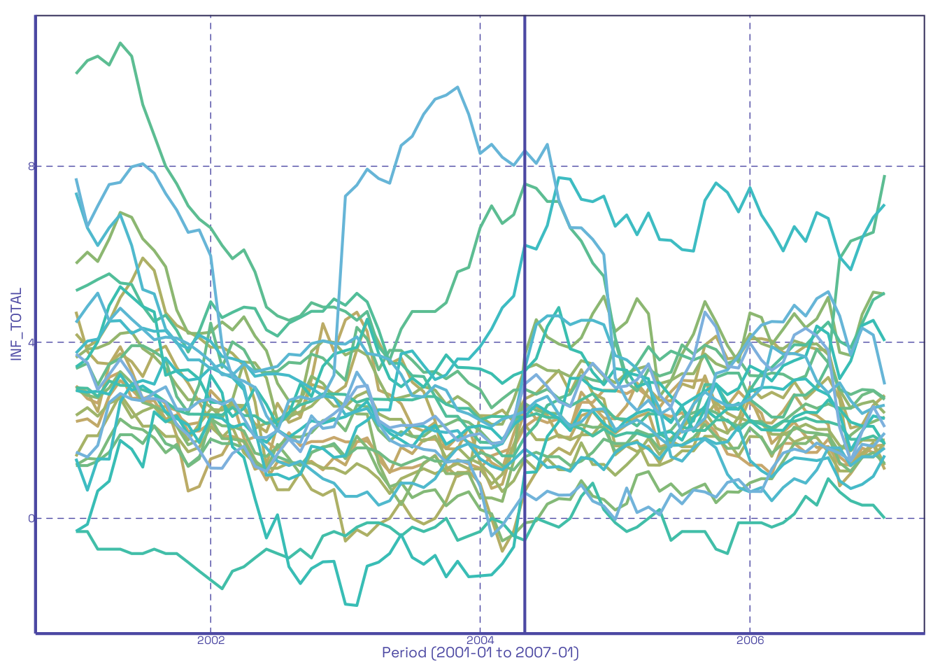
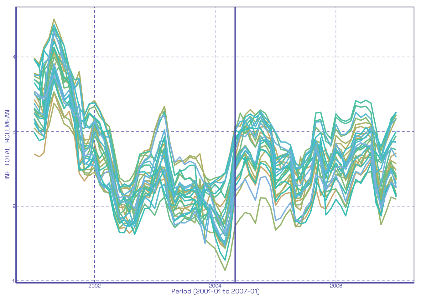
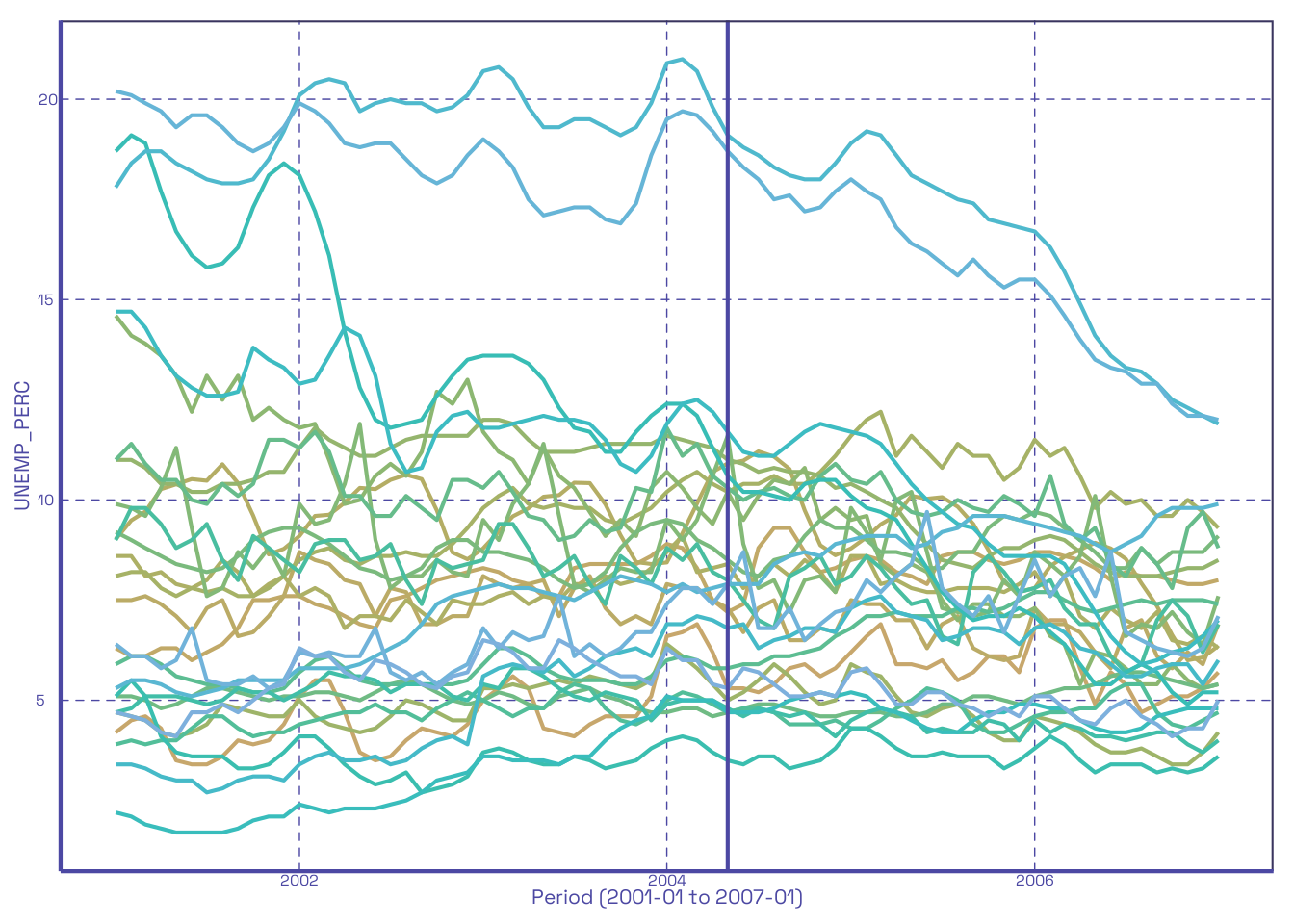
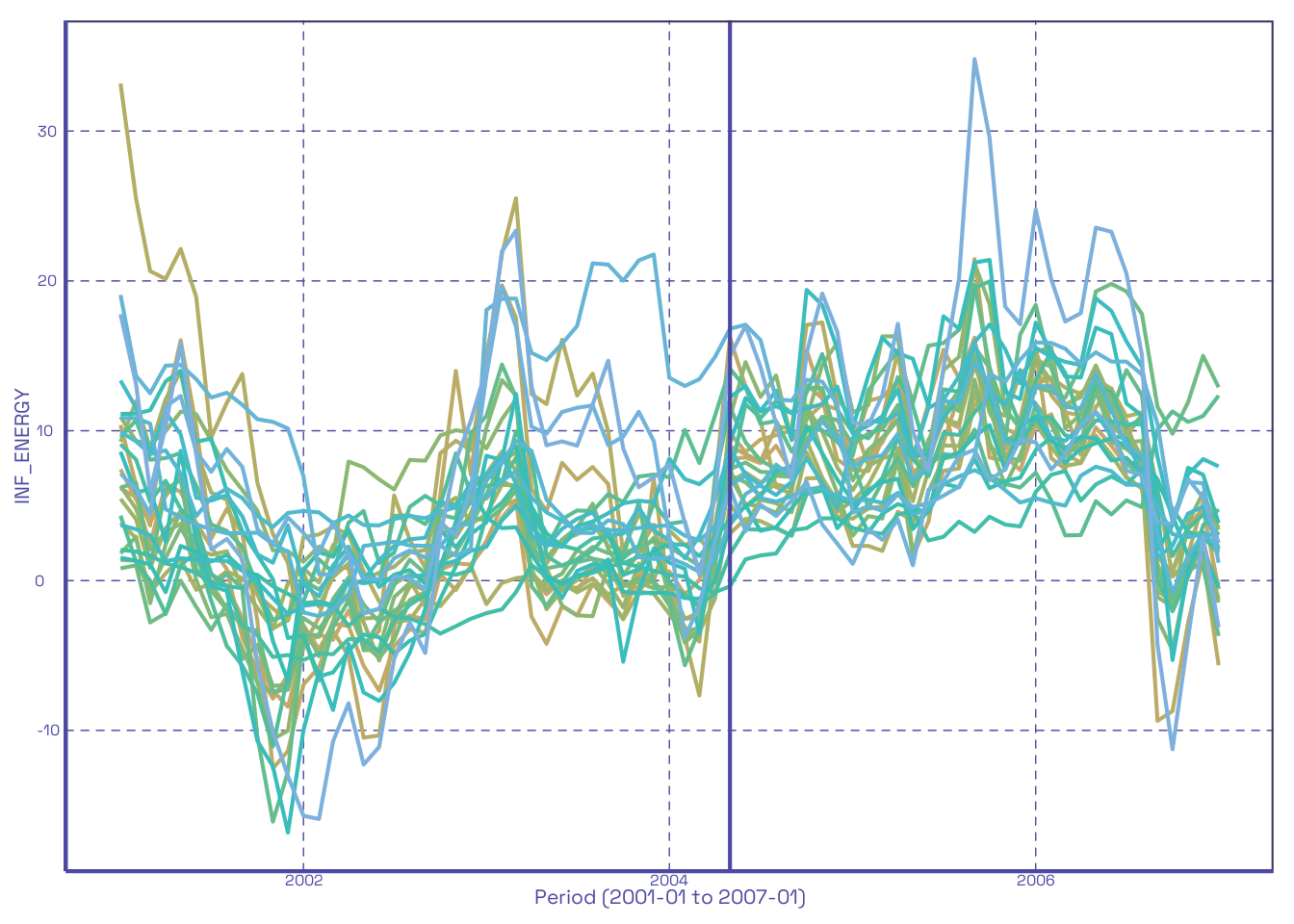
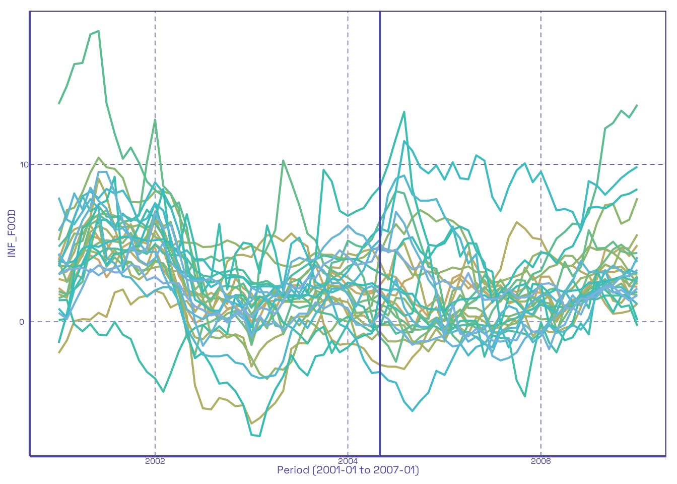
All variables have 1971 valid observations. Below is a set of plots detailing the distributions of these (numeric) variables (colored by country) in the data:

4 Model

Now to detail our model. As stated earlier, this paper implements a variation of Robert J. Gordon’s “Triangle” model of inflation. Its closest proxy is that implemented by Gordon in his 2013 working paper (Gordon 2013), but his prior published articles follow the same core elements. Gordon’s model alone, however, is not designed to consider cross-country variation (or EU membership for that matter), so we rather break up the analysis into parts:

First, we consider a baseline model (and a few slight variants), which consists of all (and then some) countries in the dataset prior to the ascension date (May 2004, n = 1056), and permits us to test the first part of the question stated in Section 1;
Second (for the second part of the question in Section 1), we consider the baseline as a panel and our countries of interest (Hungary, Poland, the Slovak Republic, Latvia, Estonia, Lithuania, and Czechia) against the rest, splitting between the pre- and post-ascension years by a dummy; and
Third, we consider a “why not do everything?” difference-in-differences implementation of the baseline model, accounting for country-level fixed-effects, EU membership, and 2004 ascension across the whole window. This is left to the appendix in Section 7.1.

In sum, we will consider many variations, largely just by restrictions and sub-setting our model data. The aim is to thoroughly demonstrate whether our expected relationship applies, and whether the expected trends among join-ers is seen.

4.1 The Baseline

Our baseline model is outlined below:

$\begin{matrix} (1) & π_{t} = M A_{t - λ}^{π} + π_{t - μ} + π_{t - ν}^{e} + π_{t - ν}^{f} + u_{t - ξ} + ε_{t} \end{matrix}$

where the parameters are defined per the notation from Section 3.1, and the subscript variables $λ$ , $μ$ , $ν$ , and $ξ$ each contain a set of values to define the lags applied to each parameter in the model. This model shares many similarities with Gordon (2013). Below is a table describing these subscripts and their associated lag values:

Model Lags
Vector	Applied To	Lags
$λ$	$M A^{π}$	1, 5, 9, 13, 17, 21
$μ$	$π$	2:4, 6:8, 10:12, 14:16, 18:20, 22:24
$ν$	$π^{e}$ , $π^{f}$	0:4
$ξ$	$u$	0:11

This method of writing the model was implemented to keep it as simple as possible to display and interpret. To see the full model in linear form, check Section 7.2 in the appendix. We shall, additionally, run this model across more restricted sets of data, first, concerning only our countries of interest, and second, variants concerning only pre-2004 ascension EU members to identify any unique results from applying different data restrictions alone. Think of it as robustness checks for some very pitiful results. All are run only for the subset period prior to May 2004.

Our parameter of interest remains the unemployment rate, $u$ , and its relationship with our outcome, as per the traditional Phillips curve relationship. The unemployment rate is collected for working-aged individuals (15 to 64) across states and is not harmonized. Per that same consideration, absent what we saw earlier in Figure 1, we would expect that the effect of unemployment on inflation is negative. Looking back at Figure 1, it is clear that some of our countries follow that trend, and with more variables included to account for some of the variation in the outcome, we could see that be generalized. But such an outcome is doubtful, and, in truth, the result is likely that the curve fails to apply in general—at least for the baseline.

There are, of course, problems with this model. Chief among them is the question of stationarity which ever-hangs over when using plain inflation as a variable. Implementing a rolling mean across some of the lags does help to assuage us of the worst fears, but even there, we can see that the means among the two (of course, given one is a mean of the other) align, and differ principally in their ranges of values and variability. Moreover, seeing as out baseline considers all countries, and does not consider variation in how unemployment reverberate throughout their respective economies (something that a time-varying unemployment gap would, in-part, handle), we are sure to see many different unemployment rates crossing many different levels of headline inflation. That would track with what we saw in Figure 1 and does not spell favorable outcomes for our first regressions. The baseline model is hampered by the fact that it is being applied to a pool of many countries and by the lack of valuable pieces of information, like the time-varying natural rates of unemployment.

4.2 Joining the EU

The model implemented for the purposes of this section is quite the same as the baseline in Equation 1, but now restricted to consider countries in two, distinct, periods and among two distinct subsets. This does not change the baseline estimating equation much, except that it treats our panel data more like a panel should we choose to run this all in one go. Per our earlier analysis, we would expect the coefficient on our parameter of interest, $u$ , remain consistent with the traditional Phillips curve relationship (assumed from Gylfason and Hochreiter (2022)), if not become more acute in that relationship. This is because: among countries not in, or not joining, the EU, they should not experience a serious change from the 2004 ascension (all else constant, and given that the states joining were not major world players), and countries that were already in the EU should have had their adjustments at whatever earlier times they joined—prior to the new wave of ascensions. In this way, countries who are not actively joining the EU, are not in the treatment group, so we split along those lines. To achieve this, we segment the data by two dummy variables (seen in Table 2): one, identifying EU membership prior to 2004 (but since 2001, pre2004member), and another identifying EU membership post-2004 (inEU2004, which is also equal to the value of pre2004member for countries prior to the ascension date). Given that our range is from 2001 to the beginning of 2007, and no countries left the EU in that period, nor did any join except in 2004, we can use these two dummies alone to successfully carve up our data as we would like (for example, the join-ers will have pre2004member + inEU2004 = 1 in the post-ascension period, whereas non-join-ers and existing members will have it = 0 and = 2, respectively). This extension will be considered with all lags to unemployment applied as in the baseline. Alongside our results from these subsets, we will apply a naive (“naive” as in, just appending a treatment and time dummy and their interaction to it) difference-in-differences variation of the model, adding terms to identify a time post ascension, and treatment (the act of joining), and the interaction of the two, to the model.

5 Empirical Analysis

5.1 The Curve

For our two principal regressions we arrive at some results meriting discussion. Below is a set of tables of coefficients¹⁰ for our variable of interest and its lags in the baseline model (with lags included) across different subsets of the data (all countries, countries of interest, and pre-2004 ascension EU members):

Table 3: Baseline Regression, Pre-2004 Ascension (Rounded to the Nearest Ten-Thousandth)

(a) All Countries, n = 1056

Variables	Coefficients (SE)
$u_{t}$	-0.0157
	(0.0105)
$u_{t - 1}$	0.0067
	(0.0087)
$u_{t - 2}$	-0.0398***
	(0.0104)
$u_{t - 3}$	-0.0606***
	(0.0104)
$u_{t - 4}$	0.0266**
	(0.0100)
$u_{t - 5}$	-0.0418***
	(0.0114)
$u_{t - 6}$	-0.0300**
	(0.0114)
$u_{t - 7}$	-0.0347**
	(0.0121)
$u_{t - 8}$	0.0341**
	(0.0107)
$u_{t - 9}$	0.0406***
	(0.0121)
$u_{t - 10}$	-0.0022
	(0.0095)
$u_{t - 11}$	-0.0454***
	(0.0100)

(b) “Join-ers”, n = 256

Variables	Coefficients (SE)
$u_{t}$	-0.0333
	(0.0354)
$u_{t - 1}$	-0.0882*
	(0.0420)
$u_{t - 2}$	0.0334
	(0.0349)
$u_{t - 3}$	0.0813+
	(0.0463)
$u_{t - 4}$	-0.0316
	(0.0390)
$u_{t - 5}$	-0.0091
	(0.0122)
$u_{t - 6}$	0.0171
	(0.0125)
$u_{t - 7}$	-0.0457
	(0.0357)
$u_{t - 8}$	0.0865*
	(0.0426)
$u_{t - 9}$	-0.0322
	(0.0356)
$u_{t - 10}$	-0.0611
	(0.0444)
$u_{t - 11}$	0.0191
	(0.0377)

Variables	Coefficients (SE)
$u_{t}$	-0.0533*
	(0.0216)
$u_{t - 1}$	0.0331+
	(0.0181)
$u_{t - 2}$	-0.0249
	(0.0165)
$u_{t - 3}$	0.03804+
	(0.0196)
$u_{t - 4}$	-0.0071
	(0.0118)
$u_{t - 5}$	-0.0681***
	(0.0137)
$u_{t - 6}$	-0.0344**
	(0.0112)
$u_{t - 7}$	-0.0059
	(0.0134)
$u_{t - 8}$	0.0205
	(0.0159)
$u_{t - 9}$	0.0005
	(0.0139)
$u_{t - 10}$	-0.0138
	(0.0136)
$u_{t - 11}$	-0.0705***
	(0.0177)

+ p < 0.1, * p < 0.05, ** p < 0.01, *** p < 0.001

Looking first at Table 3 (a), with an adjusted $R^{2}$ of 0.886. First, as noted in the footnote, all model variables were included in these regression, but the output was truncated to our parameter of interest and its lags. The full tables are available in Section 7. The coefficients on underlying inflation and its shocks were consistent with expectations based in Gordon’s prior works, and otherwise not worth much discussion. The contemporaneous unemployment term is nearly significant at the 10% level¹¹, but is not so. These results disappointingly do not tell much more than that the relationship is generally insignificant—even the distribution of coefficients through time is only in the context of our window. Per the model, all else constant, a one percentage-point increase in unemployment, $u$ , in period $t$ , would on average see a -0.016 percentage-point decline in the contemporaneous headline rate of inflation. Period $t$ would next become period $t - 1$ , where, on average and else constant, that same one percentage-point increase would see a 0.007 percentage-point increase in the headline rate of inflation. This would continue down the line for each period in time, until the the final lagged period, $t - 11$ , whereupon the average effect (if we want to roughly entertain this idea), where all else was held through all periods, totals to approximately a reduction of 0.16 percentage-points in headline inflation. This may sound like it is worth something in terms of economic significance, but that is conditioned by the fact that many of these coefficients are either: very small in magnitude, insignificant, have relatively large standard errors, or fit all of the above.

Considering a variation of Equation 1 across the same subset as Table 3 (a) that contains no lags on unemployment (only including the contemporaneous term), we arrive at a, frankly sorrowful, and entirely insignificant, coefficient of 0.0088188 on $u_{t}$ , with a standard deviation (0.0088657) larger than itself. This outcome is of course not an apples-to-apples comparison with the prior model, as we are deliberately losing some information in the process, but it helps to paint a picture of general insignificance. In fewer words, the traditional Phillips relationship fails when applied across our whole dataset, and we fail to reject the null that the rates of unemployment and inflation are particularly linked among a broad set of economies. Insignificant terms, low coefficients, and relatively high standard errors across the board.

Again, considering Figure 1, this is not a particular surprise. Similarly, if we consider a subset containing only our countries of interest Table 3 (b), the result is similarly muddled in insignificance and in fact is even worse in that respect—doing little to help the “cause of the curve” here either. One point of note that we do find in Table 3 (b), is that the first lag of unemployment is significant and of comparatively-large magnitude among other coefficients across the three tables. However, it is just as soon countered by an equally and oppositely significant coefficient on a further lag, amounting to more moot. It may be difficult to understand how puny these magnitudes are, so simply know that in Gordon (2013), the coefficient unemployment gap in his “Triangle” implementation was significant and negative at roughly -0.5, and even his New-Keynesian Phillips Curve models (largely similar, just not having all the same shocks and time-varying accessories) using the traditional unemployment rate, had coefficients that were significant and negative at roughly -0.19.

Lastly, considering a subset restricted to only include countries in the EU prior to the 2004 ascension Table 3 (c), we arrive at the least disappointing result of the three. The coefficient on the contemporaneous unemployment rate for that period is negative and significant at the 5% level—and, though still quite small in magnitude, not nearly so as the prior two cases. Most of the coefficients are negative, and a handful are significant. This is the only case where there is arguably a non-vestigial Phillips relationship. Considering the coefficients as in Table 3 (a), for a one percentage-point increase in unemployment, $u$ , in period $t$ , on average an else constant we would expect to see a decline of 0.0532792 percentage points in the rate of inflation, followed be a series of downstream lagged declines (or sometimes slight increases, although all of those are basically insignificant) in the next periods of inflation. Among some countries, surely, the curve is present, and perhaps the strongest case for applicability is the EU (despite the low magnitudes), but a rule is not a rule if you must pick and choose its applicability.

Whatever the case, it appears that the Phillips relationship is not very strong in aggregate these days, but that does not deny us a comparison between the pre- and post-periods.

5.2 The Join-ers

For this second component, we run roughly the same regression as in Table 3 (a), but expanded to include a second window period: post-2004 ascension, split by a dummy variable identifying EU membership post-2004. We include another dummy identifying EU membership in the pre-2004 period. Since we already ran one of the relevant regressions in the last section Table 3 (b), we will run the other three, compare them directly, and run a simple modified and a naive difference-in-difference models to contrast against. Below are 3 tables concerning the additional subsets (with the post-ascension period beginning with the month of ascension, May 2004):

Table 4: Comparing Coefficients, Pre-/Post-2004 Ascension Among “Join-ers” and “Non-Join-ers”

(a) “Join-ers” Post-2004, n = 207

Variables	Coefficients (SE)
$u_{t}$	0.0361668+
	(0.0190382)
$u_{t - 1}$	0.0765854***
	(0.0206344)
$u_{t - 2}$	0.0917911***
	(0.0235985)
$u_{t - 3}$	0.0501797+
	(0.0270120)
$u_{t - 4}$	-0.0177499
	(0.0271022)
$u_{t - 5}$	0.0250091+
	(0.0141664)
$u_{t - 6}$	-0.0010277
	(0.0148397)
$u_{t - 7}$	-0.0714076***
	(0.0166389)
$u_{t - 8}$	-0.1204406***
	(0.0218576)
$u_{t - 9}$	-0.0746654***
	(0.0216435)
$u_{t - 10}$	-0.0067565
	(0.0296441)
$u_{t - 11}$	0.0420206
	(0.0266813)

(b) “Non-Join-ers” Pre-2004, n = 776

Variables	Coefficients (SE)
$u_{t}$	-0.0265676
	(0.0211402)
$u_{t - 1}$	0.0071577
	(0.0143335)
$u_{t - 2}$	0.0279579*
	(0.0130221)
$u_{t - 3}$	0.0084060
	(0.0212050)
$u_{t - 4}$	0.0681393***
	(0.0172510)
$u_{t - 5}$	-0.0543169***
	(0.0140055)
$u_{t - 6}$	-0.0147423
	(0.0177657)
$u_{t - 7}$	-0.0426256**
	(0.0140238)
$u_{t - 8}$	0.0052060
	(0.0125269)
$u_{t - 9}$	-0.0383009*
	(0.0163717)
$u_{t - 10}$	0.0425551**
	(0.0162868)
$u_{t - 11}$	-0.0542168***
	(0.0144995)

Variables	Coefficients (SE)
$u_{t}$	0.0116599
	(0.0184492)
$u_{t - 1}$	0.0222061
	(0.0138293)
$u_{t - 2}$	0.0023293
	(0.0146120)
$u_{t - 3}$	-0.0023999
	(0.0201968)
$u_{t - 4}$	-0.0258058+
	(0.0139207)
$u_{t - 5}$	-0.0308985+
	(0.0171368)
$u_{t - 6}$	-0.0244802
	(0.0159395)
$u_{t - 7}$	0.0052824
	(0.0131482)
$u_{t - 8}$	-0.0389701**
	(0.0132885)
$u_{t - 9}$	-0.0145678
	(0.0174483)
$u_{t - 10}$	-0.0029622
	(0.0121239)
$u_{t - 11}$	0.0157264
	(0.0134514)

+ p < 0.1, * p < 0.05, ** p < 0.01, *** p < 0.001

From the regression outputs detailed in Table 3 (b), Table 4 (a), Table 4 (b), and Table 4 (c) we can zero in principally on the coefficients of the contemporaneous (time $t$ ) rates of unemployment across the different subsets of data. Unfortunately, we again find little evidence to support either any kind of Phillips curve relationship across subsets, and we see a clear rebuke to the second part of our question—at least when considering these subsets themselves as singly-united groups. The coefficients became more positive among joiners. A buck in the expected trend. Running a simple difference-in-differences variation of our baseline model, we see a statistically significant and negative, but again very small, coefficient on contemporaneous unemployment. But, the damning thing is the coefficient on joiners (a treatment dummy generated based on the other dummies introduced in Section 3). Not considering the interaction (which is quite small), the coefficient on the treatment dummy itself is statistically significant and large in magnitude:

Table 5: Comparing Naive DiDs

(a) Simple DiD Model Extension

Variables	Coefficients (SE)
$u_{t}$	-0.0394721***
	(0.0075784)
$u_{t - 1}$	0.0043928
	(0.0052762)
$u_{t - 2}$	-0.0111983+
	(0.0060711)
$u_{t - 3}$	-0.0411871***
	(0.0062869)
$u_{t - 4}$	0.0521342***
	(0.0069596)
$u_{t - 5}$	-0.0648863***
	(0.0068492)
$u_{t - 6}$	0.0198976**
	(0.0062217)
$u_{t - 7}$	-0.0250560***
	(0.0061447)
$u_{t - 8}$	0.0089073
	(0.0062464)
$u_{t - 9}$	0.0276457***
	(0.0063765)
$u_{t - 10}$	0.0238670***
	(0.0064501)
$u_{t - 11}$	-0.0069471
	(0.0060853)
joiners	0.8032522***
	(0.1011322)
post2004	-0.1516057**
	(0.0557524)
joiners × post2004	-0.0068386
	(0.0947133)
Num.Obs.	1947
R2	0.872
R2 Adj.	0.868
AIC	3779.7
BIC	4142.0
Log.Lik.	-1824.838
F	201.617
RMSE	0.62
Std.Errors	HC1

(b) Naive DiD Model (for reference)

Variables	Coefficients (SE)
(Intercept)	2.3132326***
	(0.0438126)
joiners	1.0920710***
	(0.1789145)
post2004	-0.1833092**
	(0.0592493)
joiners × post2004	0.7343672***
	(0.2220608)
Num.Obs.	1971
R2	0.138
R2 Adj.	0.137
AIC	7480.6
BIC	7508.5
Log.Lik.	-3735.291
F	77.362
RMSE	1.61
Std.Errors	HC1

+ p < 0.1, * p < 0.05, ** p < 0.01, *** p < 0.001

This coefficient on the treatment is just a fixed effect dummy, so it only flips on or off, but recall that the average rate of inflation across the whole data is 2.6 percentage points Table 2, and this dummy has a coefficient of 0.80. If we consider a truly naive model (as in Table 5 (b)), by contrast, governed entirely by the treatment and period dummies and their interaction, we see what Table 5 (a) hinted in its full cruelty: inflation was higher, on average, among the join-ers in the post-ascension period. This naive model is not meant to really “model” things, but rather to demonstrate the dynamics of these subsets in the simplest possible way. And what is tells us is to expect higher inflation among join-ers, and that is something supported both by our direct comparisons in Table 4 and in our (compared to the naive model) more realistic implementation in Table 5 (a).

To summarize. The Phillips relationship is not present, and even if it was, our strongest evidence from our various models suggests that join-ers saw their national rates of inflation grow upon their ascension. Considering all our model variations in sum, we find little evidence of a consistent Phillips curve relationship among any of the three primary groups: join-ers, existing members, and non-members, and find most evidence for a growth in inflation (tenuously, possibly, related to growth in unemployment, bucking the expected trend) among join-ers in the post-ascension period. If there is a traditional Phillips curve relationship to be found, this model has proved poor in ascertaining it. Our hunch, is that this is the result of missing key components of Gordon’s model that he had made serious use of. Chief among them: the time-varying rate of natural unemployment, and the unemployment gap.

As described in Section 2.3, the unemployment gap contains information on more than just labor. It is derived using the unemployment rate and core inflation, meaning that it contains information on both and varies with both through time. But it is also not sufficient to simply substitute in core inflation alongside the unemployment rate, because that overlooks their dynamic. No, there is a reason Gordon calculates the model by that method, and as noted again in Section 2.3, it demonstrably leads to results that are closer to expectations (Gordon 2013). But it is no matter, as a final extension, in the appendix, Section 7.1, we throw all the fixed-effects in the world at the model and see what that does (it helps!). But first, we shall conclude our principal findings.

6 Conclusion and Remarks

In this paper, we aimed to identify how economies of states joining the EU change with their ascensions. We did this by viewing economies through the lens of the Phillips curve relationship, implementing a variation of Robert J. Gordon’s “Triangle” model Gordon (2013) of inflation across a wide set of countries with coverage for a period of January 2001 to January 2007. In this pursuit, we first assessed the continuing validity of the traditional Phillips curve relationship and found that it is “dead,” for our purposes. Later, when we assessed how this relationship changes (by observing differences in coefficients) among subsets concerning join-ers and the rest in the pre- and post-ascension years, we found that, in contrast to the assertions of Gylfason and Hochreiter (2022), joining the EU in the 2004 phase (as Lithuania did in that paper), is, on average and else constant, consistent with higher inflation. It is possible that this particular set of years bucked some otherwise stalwart trend—but that is doubtful. It is only in our final model extension, where we apply country-level fixed effects, that we find a negative, statistically significant (at the 0.1% level), and meaningfully large(r) coefficient of -0.1058697 on the contemporaneous unemployment rate (and similar results observed among lags). At best, what this tells us is that there could be some weak underlying relationship, but this only further reinforces the notion that that relationship changed contrary to our expectations for EU join-ers.

It is difficult to consider policy implications in this context, as the model was, for reasons we have outlined, hamstrung in its utility. Applying a first-differences approach for the unemployment terms could have helped, but it was not worth delving so much deeper into extensions. Rather, we conclude to say the following: we have found little evidence to support the notion of a generally-applicable Phillips curve relationship over that time frame, and among what evidence we have gathered, it appears that EU join-ers experienced higher levels of inflation than the “untreated” non-join-ers. The EU is a hodgepodge born from post-war dreams.

7 Appendix

7.1 A DiD Diversion

As a final bit of fun, we include country-level fixed effects into the model and run a triple interaction on that term, the dummy term for EU members pre-ascension, and another dummy for members post-ascension. Including a table for this here would be a nightmare, so check Section 7 for that. But, one thing worth noting is that when looking at the fixed effects by country, the coefficient on Lithuania is quite small in magnitude (not negative, but small) among its peers. For example, the coefficient on Lithuania was insignificant at 0.1416405 with a standard error double that (0.3122093), whereas its neighbor to the North and fellow joiner Latvia had a significant coefficient of 1.6107148 with a standard error of about the same magnitude. Perhaps the assertions of Gylfason and Hochreiter (2022) are justified in the particular case of Lithuania!

7.2 The Baseline Model in Full

$π_{t} = M A_{t - 1}^{π} + π_{t - 2} + π_{t - 3} + π_{t - 4} + M A_{t - 5}^{π} + π_{t - 6} + π_{t - 7} + π_{t - 8}$

$+ M A_{t - 9}^{π} + π_{t - 10} + π_{t - 11} + π_{t - 12} + M A_{t - 13}^{π} + π_{t - 14} + π_{t - 15} + π_{t - 16}$

$\begin{matrix} (2) & + M A_{t - 17}^{π} + π_{t - 18} + π_{t - 19} + π_{t - 20} + M A_{t - 21}^{π} + π_{t - 22} + π_{t - 23} + π_{t - 24} \end{matrix}$

$+ π_{t}^{e} + π_{t - 1}^{e} + π_{t - 2}^{e} + π_{t - 3}^{e} + π_{t - 4}^{e} + π_{t}^{f} + π_{t - 1}^{f} + π_{t - 2}^{f} + π_{t - 3}^{f} + π_{t - 4}^{f}$

$+ u_{t} + u_{t - 1} + u_{t - 2} + u_{t - 3} + u_{t - 4} + u_{t - 5} + u_{t - 6} + u_{t - 7} + u_{t - 8} + u_{t - 9} + u_{t - 10} + u_{t - 11}$

Table Addendum


(Intercept)	1.3529035*
	(0.5281078)
lag(INF_TOTAL_ROLLMEAN, 1)	1.3249496***
	(0.1748481)
lag(INF_TOTAL, 2)	-0.2168568***
	(0.0335023)
lag(INF_TOTAL, 3)	0.0726361*
	(0.0327927)
lag(INF_TOTAL, 4)	-0.1864691***
	(0.0331966)
lag(INF_TOTAL_ROLLMEAN, 5)	1.9900078***
	(0.2039019)
lag(INF_TOTAL, 6)	0.0372156
	(0.0367759)
lag(INF_TOTAL, 7)	0.1120303**
	(0.0350752)
lag(INF_TOTAL, 8)	-0.0049586
	(0.0309678)
lag(INF_TOTAL_ROLLMEAN, 9)	-3.2054683***
	(0.2456334)
lag(INF_TOTAL, 10)	0.1152792***
	(0.0341819)
lag(INF_TOTAL, 11)	-0.0158565
	(0.0291393)
lag(INF_TOTAL, 12)	0.0536165*
	(0.0214169)
lag(INF_TOTAL_ROLLMEAN, 13)	0.6761022**
	(0.2477992)
lag(INF_TOTAL, 14)	0.0060775
	(0.0195168)
lag(INF_TOTAL, 15)	0.0302691
	(0.0213922)
lag(INF_TOTAL, 16)	-0.1080173***
	(0.0182163)
lag(INF_TOTAL_ROLLMEAN, 17)	2.2764730***
	(0.2313703)
lag(INF_TOTAL, 18)	-0.1062506***
	(0.0215381)
lag(INF_TOTAL, 19)	-0.0252315
	(0.0263420)
lag(INF_TOTAL, 20)	0.0543005*
	(0.0220950)
lag(INF_TOTAL_ROLLMEAN, 21)	-2.2858902***
	(0.2029851)
lag(INF_TOTAL, 22)	-0.1255131***
	(0.0238467)
lag(INF_TOTAL, 23)	0.0850301***
	(0.0242496)
lag(INF_TOTAL, 24)	0.1062509***
	(0.0226060)
INF_ENERGY	0.1192867***
	(0.0063084)
lag(INF_ENERGY, 1)	-0.0767534***
	(0.0061397)
lag(INF_ENERGY, 2)	0.0102631
	(0.0070738)
lag(INF_ENERGY, 3)	-0.0174098*
	(0.0071453)
lag(INF_ENERGY, 4)	0.0134098+
	(0.0073522)
lag(INF_ENERGY, 5)	-0.0151709*
	(0.0061205)
lag(INF_ENERGY, 6)	0.0002780
	(0.0068749)
lag(INF_ENERGY, 7)	-0.0190069**
	(0.0067933)
lag(INF_ENERGY, 8)	0.0272982***
	(0.0063649)
lag(INF_ENERGY, 9)	-0.0210499***
	(0.0059825)
lag(INF_ENERGY, 10)	-0.0204376**
	(0.0069732)
lag(INF_ENERGY, 11)	0.0260859***
	(0.0069626)
INF_FOOD	0.2625087***
	(0.0114000)
lag(INF_FOOD, 1)	-0.1142504***
	(0.0108140)
lag(INF_FOOD, 2)	-0.0040857
	(0.0125223)
lag(INF_FOOD, 3)	-0.0252051+
	(0.0141712)
lag(INF_FOOD, 4)	0.0603070***
	(0.0138935)
lag(INF_FOOD, 5)	-0.0125975
	(0.0104983)
lag(INF_FOOD, 6)	-0.0282378*
	(0.0130831)
lag(INF_FOOD, 7)	-0.0580405***
	(0.0135899)
lag(INF_FOOD, 8)	0.0363031**
	(0.0140053)
lag(INF_FOOD, 9)	0.0308544**
	(0.0112658)
lag(INF_FOOD, 10)	-0.0283568+
	(0.0150239)
lag(INF_FOOD, 11)	0.0021681
	(0.0136873)
UNEMP_PERC	-0.0156697
	(0.0104750)
lag(UNEMP_PERC, 1)	0.0067304
	(0.0086990)
lag(UNEMP_PERC, 2)	-0.0398452***
	(0.0103656)
lag(UNEMP_PERC, 3)	-0.0605775***
	(0.0103736)
lag(UNEMP_PERC, 4)	0.0265723**
	(0.0099575)
lag(UNEMP_PERC, 5)	-0.0417800***
	(0.0114164)
lag(UNEMP_PERC, 6)	0.0300209**
	(0.0107156)
lag(UNEMP_PERC, 7)	-0.0346650**
	(0.0120704)
lag(UNEMP_PERC, 8)	0.0341080**
	(0.0107439)
lag(UNEMP_PERC, 9)	0.0406185***
	(0.0121216)
lag(UNEMP_PERC, 10)	-0.0022300
	(0.0094743)
lag(UNEMP_PERC, 11)	-0.0454323***
	(0.0099781)
Num.Obs.	1056
R2	0.893
R2 Adj.	0.886
AIC	2094.1
BIC	2401.8
Log.Lik.	-985.053
RMSE	0.62
Std.Errors	HC1
p < 0.1, * p < 0.05, p < 0.01, * p < 0.001


(Intercept)	0.4316514*
	(0.1800976)
lag(INF_TOTAL_ROLLMEAN, 1)	1.2785655***
	(0.1461156)
lag(INF_TOTAL, 2)	-0.3249217***
	(0.0301856)
lag(INF_TOTAL, 3)	-0.0491959
	(0.0311894)
lag(INF_TOTAL, 4)	-0.1412934***
	(0.0335988)
lag(INF_TOTAL_ROLLMEAN, 5)	2.7295516***
	(0.1653681)
lag(INF_TOTAL, 6)	-0.0739773*
	(0.0309516)
lag(INF_TOTAL, 7)	0.0505780+
	(0.0305159)
lag(INF_TOTAL, 8)	-0.1139016***
	(0.0317402)
lag(INF_TOTAL_ROLLMEAN, 9)	-3.3514338***
	(0.2145790)
lag(INF_TOTAL, 10)	0.0032567
	(0.0324242)
lag(INF_TOTAL, 11)	-0.0899702***
	(0.0266883)
lag(INF_TOTAL, 12)	0.0299973
	(0.0195758)
lag(INF_TOTAL_ROLLMEAN, 13)	0.9513447***
	(0.2070892)
lag(INF_TOTAL, 14)	-0.0127631
	(0.0189656)
lag(INF_TOTAL, 15)	0.0143374
	(0.0190079)
lag(INF_TOTAL, 16)	-0.1100355***
	(0.0194272)
lag(INF_TOTAL_ROLLMEAN, 17)	2.2895470***
	(0.2104546)
lag(INF_TOTAL, 18)	-0.0512144*
	(0.0214659)
lag(INF_TOTAL, 19)	-0.0236584
	(0.0211595)
lag(INF_TOTAL, 20)	0.0654126**
	(0.0211989)
lag(INF_TOTAL_ROLLMEAN, 21)	-2.5820052***
	(0.1635788)
lag(INF_TOTAL, 22)	-0.0648497**
	(0.0213241)
lag(INF_TOTAL, 23)	0.0820479***
	(0.0207413)
lag(INF_TOTAL, 24)	0.1458957***
	(0.0186123)
INF_ENERGY	0.1185849***
	(0.0061782)
lag(INF_ENERGY, 1)	-0.0768545***
	(0.0062014)
lag(INF_ENERGY, 2)	0.0056246
	(0.0073491)
lag(INF_ENERGY, 3)	-0.0267785***
	(0.0074810)
lag(INF_ENERGY, 4)	0.0242841***
	(0.0071746)
lag(INF_ENERGY, 5)	-0.0217608***
	(0.0060622)
lag(INF_ENERGY, 6)	0.0051126
	(0.0069370)
lag(INF_ENERGY, 7)	-0.0207178**
	(0.0069378)
lag(INF_ENERGY, 8)	0.0348286***
	(0.0065505)
lag(INF_ENERGY, 9)	-0.0194523**
	(0.0060621)
lag(INF_ENERGY, 10)	-0.0211379**
	(0.0070600)
lag(INF_ENERGY, 11)	0.0251961***
	(0.0067739)
INF_FOOD	0.2773822***
	(0.0120351)
lag(INF_FOOD, 1)	-0.1545847***
	(0.0109061)
lag(INF_FOOD, 2)	0.0181751
	(0.0135675)
lag(INF_FOOD, 3)	-0.0144571
	(0.0146800)
lag(INF_FOOD, 4)	0.0095571
	(0.0157560)
lag(INF_FOOD, 5)	-0.0046221
	(0.0118280)
lag(INF_FOOD, 6)	-0.0033193
	(0.0137555)
lag(INF_FOOD, 7)	-0.0723082***
	(0.0143283)
lag(INF_FOOD, 8)	0.0406628**
	(0.0147903)
lag(INF_FOOD, 9)	0.0130446
	(0.0122684)
lag(INF_FOOD, 10)	-0.0144931
	(0.0159834)
lag(INF_FOOD, 11)	0.0326990*
	(0.0141316)
UNEMP_PERC	0.0088188
	(0.0088657)
Num.Obs.	1056
R2	0.860
R2 Adj.	0.853
AIC	2354.0
BIC	2607.1
Log.Lik.	-1126.007
RMSE	0.70
Std.Errors	HC1
p < 0.1, * p < 0.05, p < 0.01, * p < 0.001


(Intercept)	-0.0452176
	(0.4379585)
lag(INF_TOTAL_ROLLMEAN, 1)	0.3629458***
	(0.1060016)
lag(INF_TOTAL, 2)	-0.0528643
	(0.0552761)
lag(INF_TOTAL, 3)	-0.0858253
	(0.0787290)
lag(INF_TOTAL, 4)	0.0435107
	(0.0794619)
lag(INF_TOTAL_ROLLMEAN, 5)	-0.2943191**
	(0.0929217)
lag(INF_TOTAL, 6)	-0.0151060
	(0.0494264)
lag(INF_TOTAL, 7)	0.8012680***
	(0.0578965)
lag(INF_TOTAL, 8)	-0.0428204
	(0.0537619)
lag(INF_TOTAL_ROLLMEAN, 9)	-0.3833472***
	(0.1090815)
lag(INF_TOTAL, 10)	0.0658381
	(0.0854589)
lag(INF_TOTAL, 11)	0.0021422
	(0.0808413)
lag(INF_TOTAL, 12)	0.0813007*
	(0.0362128)
lag(INF_TOTAL_ROLLMEAN, 13)	0.1676935
	(0.1155741)
lag(INF_TOTAL, 14)	0.0227132
	(0.0358787)
lag(INF_TOTAL, 15)	-0.0171502
	(0.0446244)
lag(INF_TOTAL, 16)	-0.0778610
	(0.0482949)
lag(INF_TOTAL_ROLLMEAN, 17)	0.3830679***
	(0.1102598)
lag(INF_TOTAL, 18)	-0.0425176
	(0.0336237)
lag(INF_TOTAL, 19)	-0.0740082*
	(0.0300646)
lag(INF_TOTAL, 20)	0.0295243
	(0.0262895)
lag(INF_TOTAL_ROLLMEAN, 21)	-0.0650033
	(0.1263014)
lag(INF_TOTAL, 22)	0.0337577
	(0.0347673)
lag(INF_TOTAL, 23)	0.0410820
	(0.0289692)
lag(INF_TOTAL, 24)	0.0015971
	(0.0243413)
INF_ENERGY	0.1504089***
	(0.0169806)
lag(INF_ENERGY, 1)	-0.0139765
	(0.0093751)
lag(INF_ENERGY, 2)	0.0181869
	(0.0143245)
lag(INF_ENERGY, 3)	0.0010787
	(0.0157423)
lag(INF_ENERGY, 4)	-0.0054952
	(0.0164840)
lag(INF_ENERGY, 5)	-0.0005332
	(0.0077323)
lag(INF_ENERGY, 6)	-0.0115579
	(0.0119110)
lag(INF_ENERGY, 7)	-0.1091167***
	(0.0155009)
lag(INF_ENERGY, 8)	0.0160290
	(0.0117423)
lag(INF_ENERGY, 9)	0.0145009
	(0.0106079)
lag(INF_ENERGY, 10)	0.0026110
	(0.0177560)
lag(INF_ENERGY, 11)	0.0101329
	(0.0155530)
INF_FOOD	0.3337142***
	(0.0218207)
lag(INF_FOOD, 1)	-0.0204044
	(0.0197188)
lag(INF_FOOD, 2)	-0.0021519
	(0.0340813)
lag(INF_FOOD, 3)	0.0028374
	(0.0313289)
lag(INF_FOOD, 4)	-0.0228837
	(0.0310177)
lag(INF_FOOD, 5)	-0.0021852
	(0.0119558)
lag(INF_FOOD, 6)	-0.0121589
	(0.0191954)
lag(INF_FOOD, 7)	-0.2423173***
	(0.0269473)
lag(INF_FOOD, 8)	0.0229782
	(0.0258264)
lag(INF_FOOD, 9)	0.0361678
	(0.0332749)
lag(INF_FOOD, 10)	-0.0204948
	(0.0311093)
lag(INF_FOOD, 11)	0.0084487
	(0.0312370)
UNEMP_PERC	0.0332879
	(0.0353867)
lag(UNEMP_PERC, 1)	-0.0882479*
	(0.0420326)
lag(UNEMP_PERC, 2)	0.0333615
	(0.0348988)
lag(UNEMP_PERC, 3)	0.0812704+
	(0.0462630)
lag(UNEMP_PERC, 4)	-0.0315714
	(0.0389877)
lag(UNEMP_PERC, 5)	-0.0091083
	(0.0121778)
lag(UNEMP_PERC, 6)	0.0170697
	(0.0124964)
lag(UNEMP_PERC, 7)	-0.0457083
	(0.0357037)
lag(UNEMP_PERC, 8)	0.0864822*
	(0.0425810)
lag(UNEMP_PERC, 9)	-0.0322407
	(0.0355589)
lag(UNEMP_PERC, 10)	-0.0610766
	(0.0444125)
lag(UNEMP_PERC, 11)	0.0191295
	(0.0377118)
Num.Obs.	256
R2	0.994
R2 Adj.	0.993
AIC	56.7
BIC	276.5
Log.Lik.	33.658
RMSE	0.21
Std.Errors	HC1
p < 0.1, * p < 0.05, p < 0.01, * p < 0.001


(Intercept)	0.2564036
	(0.1691160)
lag(INF_TOTAL_ROLLMEAN, 1)	0.3202387**
	(0.1004292)
lag(INF_TOTAL, 2)	-0.0603865
	(0.0469326)
lag(INF_TOTAL, 3)	-0.0557135
	(0.0783897)
lag(INF_TOTAL, 4)	0.0762685
	(0.0751447)
lag(INF_TOTAL_ROLLMEAN, 5)	-0.2587459**
	(0.0846404)
lag(INF_TOTAL, 6)	-0.0270903
	(0.0434189)
lag(INF_TOTAL, 7)	0.8531660***
	(0.0492747)
lag(INF_TOTAL, 8)	-0.0639008
	(0.0488816)
lag(INF_TOTAL_ROLLMEAN, 9)	-0.3078151**
	(0.0986950)
lag(INF_TOTAL, 10)	0.0418111
	(0.0817076)
lag(INF_TOTAL, 11)	-0.0065448
	(0.0808650)
lag(INF_TOTAL, 12)	0.0788421*
	(0.0340149)
lag(INF_TOTAL_ROLLMEAN, 13)	0.1570926
	(0.1016114)
lag(INF_TOTAL, 14)	0.0152597
	(0.0353234)
lag(INF_TOTAL, 15)	-0.0172717
	(0.0435268)
lag(INF_TOTAL, 16)	-0.0701431
	(0.0473175)
lag(INF_TOTAL_ROLLMEAN, 17)	0.3372942**
	(0.1119870)
lag(INF_TOTAL, 18)	-0.0270332
	(0.0359386)
lag(INF_TOTAL, 19)	-0.0667368*
	(0.0291894)
lag(INF_TOTAL, 20)	0.0306340
	(0.0262349)
lag(INF_TOTAL_ROLLMEAN, 21)	-0.1032837
	(0.1222615)
lag(INF_TOTAL, 22)	0.0311395
	(0.0316569)
lag(INF_TOTAL, 23)	0.0456008
	(0.0278740)
lag(INF_TOTAL, 24)	-0.0067595
	(0.0249427)
INF_ENERGY	0.1577339***
	(0.0189911)
lag(INF_ENERGY, 1)	-0.0127212
	(0.0089599)
lag(INF_ENERGY, 2)	0.0133102
	(0.0135403)
lag(INF_ENERGY, 3)	-0.0027235
	(0.0161845)
lag(INF_ENERGY, 4)	-0.0147950
	(0.0158503)
lag(INF_ENERGY, 5)	-0.0024493
	(0.0066108)
lag(INF_ENERGY, 6)	-0.0076691
	(0.0091177)
lag(INF_ENERGY, 7)	-0.1212887***
	(0.0179268)
lag(INF_ENERGY, 8)	0.0202061+
	(0.0110510)
lag(INF_ENERGY, 9)	0.0136453
	(0.0111899)
lag(INF_ENERGY, 10)	0.0134602
	(0.0178902)
lag(INF_ENERGY, 11)	0.0067241
	(0.0149345)
INF_FOOD	0.3394153***
	(0.0224186)
lag(INF_FOOD, 1)	-0.0329152
	(0.0205163)
lag(INF_FOOD, 2)	-0.0034768
	(0.0346376)
lag(INF_FOOD, 3)	0.0061191
	(0.0312145)
lag(INF_FOOD, 4)	-0.0355175
	(0.0296010)
lag(INF_FOOD, 5)	-0.0027979
	(0.0101547)
lag(INF_FOOD, 6)	-0.0110415
	(0.0177467)
lag(INF_FOOD, 7)	-0.2650452***
	(0.0263257)
lag(INF_FOOD, 8)	0.0445181+
	(0.0245738)
lag(INF_FOOD, 9)	0.0329996
	(0.0346295)
lag(INF_FOOD, 10)	-0.0228566
	(0.0293025)
lag(INF_FOOD, 11)	0.0174912
	(0.0298435)
UNEMP_PERC	-0.0247369*
	(0.0102615)
Num.Obs.	256
R2	0.994
R2 Adj.	0.992
AIC	57.9
BIC	238.7
Log.Lik.	22.070
RMSE	0.22
Std.Errors	HC1
p < 0.1, * p < 0.05, p < 0.01, * p < 0.001


(Intercept)	1.7351512***
	(0.4771274)
lag(INF_TOTAL_ROLLMEAN, 1)	0.2458390*
	(0.0996931)
lag(INF_TOTAL, 2)	0.1225137***
	(0.0307948)
lag(INF_TOTAL, 3)	0.0091152
	(0.0699098)
lag(INF_TOTAL, 4)	-0.0329110
	(0.0543982)
lag(INF_TOTAL_ROLLMEAN, 5)	0.0352451
	(0.0819316)
lag(INF_TOTAL, 6)	-0.1460626***
	(0.0400850)
lag(INF_TOTAL, 7)	-0.0199802
	(0.0426907)
lag(INF_TOTAL, 8)	0.0356981
	(0.0480489)
lag(INF_TOTAL_ROLLMEAN, 9)	0.1923896**
	(0.0726238)
lag(INF_TOTAL, 10)	0.0302243
	(0.0337180)
lag(INF_TOTAL, 11)	0.0291821
	(0.0298520)
lag(INF_TOTAL, 12)	0.0129406
	(0.0419526)
lag(INF_TOTAL_ROLLMEAN, 13)	-0.2264389**
	(0.0726857)
lag(INF_TOTAL, 14)	0.0512401
	(0.0324672)
lag(INF_TOTAL, 15)	0.6050849***
	(0.0436398)
lag(INF_TOTAL, 16)	0.0174824
	(0.0300547)
lag(INF_TOTAL_ROLLMEAN, 17)	-0.0975812
	(0.0899475)
lag(INF_TOTAL, 18)	0.0093313
	(0.0595865)
lag(INF_TOTAL, 19)	0.0388806
	(0.0378942)
lag(INF_TOTAL, 20)	0.0503761*
	(0.0245409)
lag(INF_TOTAL_ROLLMEAN, 21)	-0.2620071**
	(0.0811757)
lag(INF_TOTAL, 22)	0.0550275
	(0.0423247)
lag(INF_TOTAL, 23)	0.0165576
	(0.0434042)
lag(INF_TOTAL, 24)	-0.0291167
	(0.0263767)
INF_ENERGY	0.0513622***
	(0.0063611)
lag(INF_ENERGY, 1)	-0.0106758+
	(0.0064674)
lag(INF_ENERGY, 2)	-0.0028033
	(0.0063207)
lag(INF_ENERGY, 3)	0.0017777
	(0.0069856)
lag(INF_ENERGY, 4)	0.0090399
	(0.0061333)
lag(INF_ENERGY, 5)	-0.0010528
	(0.0052839)
lag(INF_ENERGY, 6)	-0.0041853
	(0.0055549)
lag(INF_ENERGY, 7)	0.0091051
	(0.0060665)
lag(INF_ENERGY, 8)	-0.0179500**
	(0.0056588)
lag(INF_ENERGY, 9)	0.0075889
	(0.0057231)
lag(INF_ENERGY, 10)	-0.0048306
	(0.0059045)
lag(INF_ENERGY, 11)	-0.0175170**
	(0.0065681)
INF_FOOD	0.1529120***
	(0.0168775)
lag(INF_FOOD, 1)	-0.0380459**
	(0.0136196)
lag(INF_FOOD, 2)	-0.0149221
	(0.0122142)
lag(INF_FOOD, 3)	-0.0148866
	(0.0140508)
lag(INF_FOOD, 4)	-0.0139770
	(0.0166822)
lag(INF_FOOD, 5)	-0.0185971+
	(0.0112080)
lag(INF_FOOD, 6)	0.0145583
	(0.0133615)
lag(INF_FOOD, 7)	0.0130098
	(0.0163394)
lag(INF_FOOD, 8)	-0.0019446
	(0.0116834)
lag(INF_FOOD, 9)	0.0058866
	(0.0133890)
lag(INF_FOOD, 10)	-0.0128802
	(0.0138698)
lag(INF_FOOD, 11)	-0.0191824
	(0.0123224)
UNEMP_PERC	-0.0532792*
	(0.0216181)
lag(UNEMP_PERC, 1)	0.0330620+
	(0.0181012)
lag(UNEMP_PERC, 2)	-0.0248874
	(0.0165103)
lag(UNEMP_PERC, 3)	0.0380454+
	(0.0195513)
lag(UNEMP_PERC, 4)	-0.0070666
	(0.0118407)
lag(UNEMP_PERC, 5)	-0.0681305***
	(0.0136653)
lag(UNEMP_PERC, 6)	-0.0343692**
	(0.0111703)
lag(UNEMP_PERC, 7)	-0.0058717
	(0.0133609)
lag(UNEMP_PERC, 8)	0.0205142
	(0.0158614)
lag(UNEMP_PERC, 9)	0.0004827
	(0.0139474)
lag(UNEMP_PERC, 10)	-0.0137814
	(0.0136290)
lag(UNEMP_PERC, 11)	-0.0704648***
	(0.0177143)
Num.Obs.	576
R2	0.924
R2 Adj.	0.916
AIC	332.4
BIC	602.5
Log.Lik.	-104.200
RMSE	0.29
Std.Errors	HC1
p < 0.1, * p < 0.05, p < 0.01, * p < 0.001


(Intercept)	0.2668171+
	(0.1420919)
lag(INF_TOTAL_ROLLMEAN, 1)	0.0914395
	(0.0938652)
lag(INF_TOTAL, 2)	0.1087950***
	(0.0319839)
lag(INF_TOTAL, 3)	-0.0522873
	(0.0907554)
lag(INF_TOTAL, 4)	0.0064327
	(0.0464601)
lag(INF_TOTAL_ROLLMEAN, 5)	0.2164375*
	(0.0903113)
lag(INF_TOTAL, 6)	-0.0653279*
	(0.0303769)
lag(INF_TOTAL, 7)	0.0448334
	(0.0419096)
lag(INF_TOTAL, 8)	0.0059995
	(0.0453526)
lag(INF_TOTAL_ROLLMEAN, 9)	0.0554844
	(0.0641981)
lag(INF_TOTAL, 10)	0.0375807
	(0.0338259)
lag(INF_TOTAL, 11)	0.0175742
	(0.0279498)
lag(INF_TOTAL, 12)	-0.0326959
	(0.0370780)
lag(INF_TOTAL_ROLLMEAN, 13)	-0.0247558
	(0.0651764)
lag(INF_TOTAL, 14)	0.0769701**
	(0.0278410)
lag(INF_TOTAL, 15)	0.6591875***
	(0.0396576)
lag(INF_TOTAL, 16)	0.0456091
	(0.0343724)
lag(INF_TOTAL_ROLLMEAN, 17)	-0.1454626*
	(0.0735708)
lag(INF_TOTAL, 18)	0.0045515
	(0.0767198)
lag(INF_TOTAL, 19)	0.0633145
	(0.0429900)
lag(INF_TOTAL, 20)	0.0447787+
	(0.0254745)
lag(INF_TOTAL_ROLLMEAN, 21)	-0.2539177**
	(0.0794429)
lag(INF_TOTAL, 22)	0.0112237
	(0.0444276)
lag(INF_TOTAL, 23)	0.0020158
	(0.0405911)
lag(INF_TOTAL, 24)	-0.0251689
	(0.0254116)
INF_ENERGY	0.0474310***
	(0.0067923)
lag(INF_ENERGY, 1)	-0.0086128
	(0.0067918)
lag(INF_ENERGY, 2)	-0.0021854
	(0.0068115)
lag(INF_ENERGY, 3)	0.0032667
	(0.0074289)
lag(INF_ENERGY, 4)	0.0084144
	(0.0063243)
lag(INF_ENERGY, 5)	0.0012142
	(0.0060163)
lag(INF_ENERGY, 6)	-0.0145551*
	(0.0060318)
lag(INF_ENERGY, 7)	0.0130964*
	(0.0065396)
lag(INF_ENERGY, 8)	-0.0147715**
	(0.0054502)
lag(INF_ENERGY, 9)	-0.0018190
	(0.0054283)
lag(INF_ENERGY, 10)	-0.0057448
	(0.0061974)
lag(INF_ENERGY, 11)	-0.0160731*
	(0.0066973)
INF_FOOD	0.1470942***
	(0.0191319)
lag(INF_FOOD, 1)	-0.0450836**
	(0.0144340)
lag(INF_FOOD, 2)	-0.0194020
	(0.0129556)
lag(INF_FOOD, 3)	-0.0083150
	(0.0135533)
lag(INF_FOOD, 4)	-0.0137235
	(0.0165289)
lag(INF_FOOD, 5)	-0.0050070
	(0.0115749)
lag(INF_FOOD, 6)	-0.0024554
	(0.0131210)
lag(INF_FOOD, 7)	-0.0186432
	(0.0159342)
lag(INF_FOOD, 8)	0.0101599
	(0.0117943)
lag(INF_FOOD, 9)	0.0098717
	(0.0136829)
lag(INF_FOOD, 10)	-0.0233967
	(0.0148187)
lag(INF_FOOD, 11)	0.0105691
	(0.0126578)
UNEMP_PERC	-0.0214106+
	(0.0124705)
Num.Obs.	576
R2	0.910
R2 Adj.	0.902
AIC	410.4
BIC	632.5
Log.Lik.	-154.184
RMSE	0.32
Std.Errors	HC1
p < 0.1, * p < 0.05, p < 0.01, * p < 0.001


(Intercept)	0.6273218
	(0.4851352)
lag(INF_TOTAL_ROLLMEAN, 1)	0.5021741***
	(0.1264182)
lag(INF_TOTAL, 2)	0.1228035*
	(0.0583957)
lag(INF_TOTAL, 3)	-0.0335518
	(0.0566738)
lag(INF_TOTAL, 4)	-0.0088619
	(0.0571717)
lag(INF_TOTAL_ROLLMEAN, 5)	-0.0140198
	(0.0848928)
lag(INF_TOTAL, 6)	0.0627312*
	(0.0266130)
lag(INF_TOTAL, 7)	-0.0370802
	(0.0301229)
lag(INF_TOTAL, 8)	-0.0024935
	(0.0341049)
lag(INF_TOTAL_ROLLMEAN, 9)	0.0224188
	(0.0802757)
lag(INF_TOTAL, 10)	0.0818113**
	(0.0267256)
lag(INF_TOTAL, 11)	-0.0150841
	(0.0349614)
lag(INF_TOTAL, 12)	0.0423870+
	(0.0227849)
lag(INF_TOTAL_ROLLMEAN, 13)	0.0875582
	(0.0781703)
lag(INF_TOTAL, 14)	0.0050478
	(0.0240563)
lag(INF_TOTAL, 15)	0.0643161*
	(0.0262085)
lag(INF_TOTAL, 16)	0.0439573
	(0.0285832)
lag(INF_TOTAL_ROLLMEAN, 17)	-0.1196562
	(0.1129146)
lag(INF_TOTAL, 18)	-0.0208523
	(0.0236197)
lag(INF_TOTAL, 19)	0.0450522+
	(0.0270071)
lag(INF_TOTAL, 20)	0.5860130***
	(0.0458103)
lag(INF_TOTAL_ROLLMEAN, 21)	-0.4565590***
	(0.1112014)
lag(INF_TOTAL, 22)	-0.1005759+
	(0.0514406)
lag(INF_TOTAL, 23)	0.0017727
	(0.0483007)
lag(INF_TOTAL, 24)	0.0662661
	(0.0429781)
INF_ENERGY	0.0404108***
	(0.0064715)
lag(INF_ENERGY, 1)	-0.0057705
	(0.0049540)
lag(INF_ENERGY, 2)	0.0076768
	(0.0060701)
lag(INF_ENERGY, 3)	-0.0079685
	(0.0052366)
lag(INF_ENERGY, 4)	-0.0016268
	(0.0053501)
lag(INF_ENERGY, 5)	0.0063784+
	(0.0037490)
lag(INF_ENERGY, 6)	-0.0265555***
	(0.0052464)
lag(INF_ENERGY, 7)	0.0168151***
	(0.0048590)
lag(INF_ENERGY, 8)	-0.0107321*
	(0.0052553)
lag(INF_ENERGY, 9)	-0.0082503*
	(0.0039956)
lag(INF_ENERGY, 10)	0.0005724
	(0.0050673)
lag(INF_ENERGY, 11)	-0.0065200
	(0.0048775)
INF_FOOD	0.1474098***
	(0.0164159)
lag(INF_FOOD, 1)	-0.0050147
	(0.0096841)
lag(INF_FOOD, 2)	-0.0393449**
	(0.0127624)
lag(INF_FOOD, 3)	0.0132780
	(0.0112190)
lag(INF_FOOD, 4)	-0.0131168
	(0.0122335)
lag(INF_FOOD, 5)	-0.0049099
	(0.0084910)
lag(INF_FOOD, 6)	-0.0356945**
	(0.0127448)
lag(INF_FOOD, 7)	0.0003513
	(0.0114128)
lag(INF_FOOD, 8)	0.0162938
	(0.0115566)
lag(INF_FOOD, 9)	-0.0090758
	(0.0096568)
lag(INF_FOOD, 10)	-0.0474059***
	(0.0131680)
lag(INF_FOOD, 11)	-0.0193296
	(0.0140250)
UNEMP_PERC	-0.0265676
	(0.0211402)
lag(UNEMP_PERC, 1)	0.0071577
	(0.0143335)
lag(UNEMP_PERC, 2)	0.0279579*
	(0.0130221)
lag(UNEMP_PERC, 3)	0.0084060
	(0.0212050)
lag(UNEMP_PERC, 4)	0.0681393***
	(0.0172510)
lag(UNEMP_PERC, 5)	-0.0543169***
	(0.0140055)
lag(UNEMP_PERC, 6)	-0.0147423
	(0.0177657)
lag(UNEMP_PERC, 7)	-0.0426256**
	(0.0140238)
lag(UNEMP_PERC, 8)	0.0052060
	(0.0125269)
lag(UNEMP_PERC, 9)	-0.0383009*
	(0.0163717)
lag(UNEMP_PERC, 10)	0.0425551**
	(0.0162868)
lag(UNEMP_PERC, 11)	-0.0542168***
	(0.0144995)
Num.Obs.	776
R2	0.910
R2 Adj.	0.902
AIC	788.9
BIC	1077.4
Log.Lik.	-332.426
RMSE	0.37
Std.Errors	HC1
p < 0.1, * p < 0.05, p < 0.01, * p < 0.001


(Intercept)	0.9969765+
	(0.5139871)
lag(INF_TOTAL_ROLLMEAN, 1)	0.6755992***
	(0.1073093)
lag(INF_TOTAL, 2)	-0.0970308
	(0.0640951)
lag(INF_TOTAL, 3)	-0.0406554
	(0.0547872)
lag(INF_TOTAL, 4)	0.0294030
	(0.0403076)
lag(INF_TOTAL_ROLLMEAN, 5)	0.0043589
	(0.0808910)
lag(INF_TOTAL, 6)	0.0693290*
	(0.0293053)
lag(INF_TOTAL, 7)	-0.0034040
	(0.0273216)
lag(INF_TOTAL, 8)	0.0234103
	(0.0254954)
lag(INF_TOTAL_ROLLMEAN, 9)	0.0686533
	(0.0700966)
lag(INF_TOTAL, 10)	0.0221431
	(0.0244261)
lag(INF_TOTAL, 11)	0.0239375
	(0.0212583)
lag(INF_TOTAL, 12)	-0.0302864
	(0.0221318)
lag(INF_TOTAL_ROLLMEAN, 13)	-0.1738134*
	(0.0688636)
lag(INF_TOTAL, 14)	0.0676243***
	(0.0195393)
lag(INF_TOTAL, 15)	-0.0142866
	(0.0213500)
lag(INF_TOTAL, 16)	0.0234579
	(0.0234710)
lag(INF_TOTAL_ROLLMEAN, 17)	-0.0492920
	(0.0810794)
lag(INF_TOTAL, 18)	0.0000937
	(0.0221614)
lag(INF_TOTAL, 19)	-0.0512023*
	(0.0237313)
lag(INF_TOTAL, 20)	0.6955310***
	(0.0335364)
lag(INF_TOTAL_ROLLMEAN, 21)	-0.5292360***
	(0.1123615)
lag(INF_TOTAL, 22)	0.0572754
	(0.0566548)
lag(INF_TOTAL, 23)	0.0263970
	(0.0493325)
lag(INF_TOTAL, 24)	-0.0293839
	(0.0355517)
INF_ENERGY	0.0457584***
	(0.0050268)
lag(INF_ENERGY, 1)	-0.0014996
	(0.0033604)
lag(INF_ENERGY, 2)	-0.0004538
	(0.0046644)
lag(INF_ENERGY, 3)	-0.0126453*
	(0.0055734)
lag(INF_ENERGY, 4)	-0.0053440
	(0.0048225)
lag(INF_ENERGY, 5)	0.0040031
	(0.0046519)
lag(INF_ENERGY, 6)	-0.0187350***
	(0.0049893)
lag(INF_ENERGY, 7)	-0.0107597*
	(0.0052875)
lag(INF_ENERGY, 8)	0.0014852
	(0.0047494)
lag(INF_ENERGY, 9)	0.0048444
	(0.0049683)
lag(INF_ENERGY, 10)	-0.0045124
	(0.0043792)
lag(INF_ENERGY, 11)	0.0091670+
	(0.0050896)
INF_FOOD	0.0683368***
	(0.0100508)
lag(INF_FOOD, 1)	0.0152464
	(0.0105096)
lag(INF_FOOD, 2)	-0.0012854
	(0.0094982)
lag(INF_FOOD, 3)	-0.0173732
	(0.0116810)
lag(INF_FOOD, 4)	-0.0100584
	(0.0107304)
lag(INF_FOOD, 5)	-0.0151757
	(0.0095866)
lag(INF_FOOD, 6)	-0.0254880**
	(0.0098133)
lag(INF_FOOD, 7)	-0.0175085+
	(0.0095179)
lag(INF_FOOD, 8)	-0.0165441
	(0.0105791)
lag(INF_FOOD, 9)	0.0109588
	(0.0090454)
lag(INF_FOOD, 10)	0.0023382
	(0.0107593)
lag(INF_FOOD, 11)	-0.0084762
	(0.0117746)
UNEMP_PERC	0.0116599
	(0.0184492)
lag(UNEMP_PERC, 1)	0.0222061
	(0.0138293)
lag(UNEMP_PERC, 2)	0.0023293
	(0.0146120)
lag(UNEMP_PERC, 3)	-0.0023999
	(0.0201968)
lag(UNEMP_PERC, 4)	-0.0258058+
	(0.0139207)
lag(UNEMP_PERC, 5)	-0.0308985+
	(0.0171368)
lag(UNEMP_PERC, 6)	-0.0244802
	(0.0159395)
lag(UNEMP_PERC, 7)	0.0052824
	(0.0131482)
lag(UNEMP_PERC, 8)	-0.0389701**
	(0.0132885)
lag(UNEMP_PERC, 9)	-0.0145678
	(0.0174483)
lag(UNEMP_PERC, 10)	-0.0029622
	(0.0121239)
lag(UNEMP_PERC, 11)	0.0157264
	(0.0134514)
Num.Obs.	636
R2	0.931
R2 Adj.	0.924
AIC	257.9
BIC	534.1
Log.Lik.	-66.942
RMSE	0.27
Std.Errors	HC1
p < 0.1, * p < 0.05, p < 0.01, * p < 0.001


(Intercept)	-0.4043496
	(0.3577975)
lag(INF_TOTAL_ROLLMEAN, 1)	0.1070832
	(0.1299992)
lag(INF_TOTAL, 2)	-0.0830658
	(0.0526828)
lag(INF_TOTAL, 3)	-0.0381181
	(0.0918830)
lag(INF_TOTAL, 4)	-0.0485881
	(0.0668447)
lag(INF_TOTAL_ROLLMEAN, 5)	0.0697864
	(0.1399162)
lag(INF_TOTAL, 6)	-0.1086397+
	(0.0603239)
lag(INF_TOTAL, 7)	0.7365635***
	(0.0616495)
lag(INF_TOTAL, 8)	-0.0864132
	(0.0524488)
lag(INF_TOTAL_ROLLMEAN, 9)	0.0782504
	(0.1582641)
lag(INF_TOTAL, 10)	0.0100979
	(0.0969943)
lag(INF_TOTAL, 11)	0.0003022
	(0.0742200)
lag(INF_TOTAL, 12)	0.0365727
	(0.0263707)
lag(INF_TOTAL_ROLLMEAN, 13)	0.0785277
	(0.1172145)
lag(INF_TOTAL, 14)	-0.0012088
	(0.0242490)
lag(INF_TOTAL, 15)	0.0053537
	(0.0204719)
lag(INF_TOTAL, 16)	0.0366197
	(0.0242669)
lag(INF_TOTAL_ROLLMEAN, 17)	0.0001527
	(0.1366521)
lag(INF_TOTAL, 18)	0.0062755
	(0.0219835)
lag(INF_TOTAL, 19)	-0.0039616
	(0.0222303)
lag(INF_TOTAL, 20)	-0.0099878
	(0.0203328)
lag(INF_TOTAL_ROLLMEAN, 21)	0.0133846
	(0.1093821)
lag(INF_TOTAL, 22)	0.0157168
	(0.0259488)
lag(INF_TOTAL, 23)	-0.0193103
	(0.0187869)
lag(INF_TOTAL, 24)	-0.0584624**
	(0.0190475)
INF_ENERGY	0.1724430***
	(0.0110624)
lag(INF_ENERGY, 1)	0.0136616
	(0.0085025)
lag(INF_ENERGY, 2)	0.0109559
	(0.0148231)
lag(INF_ENERGY, 3)	0.0044826
	(0.0167039)
lag(INF_ENERGY, 4)	0.0045943
	(0.0127666)
lag(INF_ENERGY, 5)	-0.0173300*
	(0.0084349)
lag(INF_ENERGY, 6)	0.0246885
	(0.0163620)
lag(INF_ENERGY, 7)	-0.1103235***
	(0.0147087)
lag(INF_ENERGY, 8)	-0.0033563
	(0.0116295)
lag(INF_ENERGY, 9)	-0.0225929*
	(0.0099434)
lag(INF_ENERGY, 10)	-0.0022879
	(0.0173212)
lag(INF_ENERGY, 11)	-0.0012431
	(0.0150341)
INF_FOOD	0.2829333***
	(0.0171604)
lag(INF_FOOD, 1)	-0.0278740
	(0.0173527)
lag(INF_FOOD, 2)	0.0367520+
	(0.0207138)
lag(INF_FOOD, 3)	0.0145680
	(0.0314548)
lag(INF_FOOD, 4)	0.0054962
	(0.0286467)
lag(INF_FOOD, 5)	-0.0070781
	(0.0133061)
lag(INF_FOOD, 6)	0.0586529***
	(0.0173283)
lag(INF_FOOD, 7)	-0.2053541***
	(0.0226998)
lag(INF_FOOD, 8)	0.0405272+
	(0.0230257)
lag(INF_FOOD, 9)	0.0016346
	(0.0147595)
lag(INF_FOOD, 10)	0.0191893
	(0.0319968)
lag(INF_FOOD, 11)	0.0143279
	(0.0285022)
UNEMP_PERC	0.0361668+
	(0.0190382)
lag(UNEMP_PERC, 1)	0.0765854***
	(0.0206344)
lag(UNEMP_PERC, 2)	0.0917911***
	(0.0235985)
lag(UNEMP_PERC, 3)	0.0501797+
	(0.0270120)
lag(UNEMP_PERC, 4)	-0.0177499
	(0.0271022)
lag(UNEMP_PERC, 5)	0.0250091+
	(0.0141664)
lag(UNEMP_PERC, 6)	-0.0010277
	(0.0148397)
lag(UNEMP_PERC, 7)	-0.0714076***
	(0.0166389)
lag(UNEMP_PERC, 8)	-0.1204406***
	(0.0218576)
lag(UNEMP_PERC, 9)	-0.0746654***
	(0.0216435)
lag(UNEMP_PERC, 10)	-0.0067565
	(0.0296441)
lag(UNEMP_PERC, 11)	0.0420206
	(0.0266813)
Num.Obs.	207
R2	0.992
R2 Adj.	0.989
AIC	-47.2
BIC	159.4
Log.Lik.	85.596
RMSE	0.16
Std.Errors	HC1
p < 0.1, * p < 0.05, p < 0.01, * p < 0.001


(Intercept)	0.6894247**
	(0.2540804)
lag(INF_TOTAL_ROLLMEAN, 1)	0.9376072***
	(0.1198447)
lag(INF_TOTAL, 2)	-0.2597413***
	(0.0226906)
lag(INF_TOTAL, 3)	0.0407956+
	(0.0224662)
lag(INF_TOTAL, 4)	-0.0840737***
	(0.0233495)
lag(INF_TOTAL_ROLLMEAN, 5)	2.1956614***
	(0.1393396)
lag(INF_TOTAL, 6)	0.0790290**
	(0.0257046)
lag(INF_TOTAL, 7)	0.0377956
	(0.0241556)
lag(INF_TOTAL, 8)	0.0399633+
	(0.0242279)
lag(INF_TOTAL_ROLLMEAN, 9)	-3.1626925***
	(0.1786538)
lag(INF_TOTAL, 10)	0.0705074**
	(0.0252043)
lag(INF_TOTAL, 11)	-0.0600537**
	(0.0210306)
lag(INF_TOTAL, 12)	0.0350344*
	(0.0161836)
lag(INF_TOTAL_ROLLMEAN, 13)	0.6301856***
	(0.1598030)
lag(INF_TOTAL, 14)	0.0023871
	(0.0143397)
lag(INF_TOTAL, 15)	-0.0670245***
	(0.0157232)
lag(INF_TOTAL, 16)	-0.1246035***
	(0.0136069)
lag(INF_TOTAL_ROLLMEAN, 17)	2.2844696***
	(0.1645936)
lag(INF_TOTAL, 18)	-0.0643472***
	(0.0142452)
lag(INF_TOTAL, 19)	-0.0544308***
	(0.0150875)
lag(INF_TOTAL, 20)	0.0211338
	(0.0150963)
lag(INF_TOTAL_ROLLMEAN, 21)	-1.8818518***
	(0.1341277)
lag(INF_TOTAL, 22)	-0.1060873***
	(0.0176548)
lag(INF_TOTAL, 23)	0.0561977***
	(0.0146639)
lag(INF_TOTAL, 24)	0.1115280***
	(0.0153477)
INF_ENERGY	0.1038653***
	(0.0044712)
lag(INF_ENERGY, 1)	-0.0501568***
	(0.0044310)
lag(INF_ENERGY, 2)	0.0012888
	(0.0047091)
lag(INF_ENERGY, 3)	-0.0162080**
	(0.0051169)
lag(INF_ENERGY, 4)	0.0129178**
	(0.0047439)
lag(INF_ENERGY, 5)	-0.0042787
	(0.0043012)
lag(INF_ENERGY, 6)	-0.0125332*
	(0.0049098)
lag(INF_ENERGY, 7)	-0.0028147
	(0.0047640)
lag(INF_ENERGY, 8)	0.0095672*
	(0.0046514)
lag(INF_ENERGY, 9)	-0.0188968***
	(0.0041051)
lag(INF_ENERGY, 10)	-0.0090541+
	(0.0046913)
lag(INF_ENERGY, 11)	0.0157031***
	(0.0045206)
INF_FOOD	0.2560591***
	(0.0082334)
lag(INF_FOOD, 1)	-0.1190935***
	(0.0072723)
lag(INF_FOOD, 2)	0.0188258*
	(0.0090392)
lag(INF_FOOD, 3)	-0.0243214*
	(0.0100497)
lag(INF_FOOD, 4)	0.0326679***
	(0.0098521)
lag(INF_FOOD, 5)	-0.0028758
	(0.0073319)
lag(INF_FOOD, 6)	-0.0409708***
	(0.0098644)
lag(INF_FOOD, 7)	-0.0306215**
	(0.0101235)
lag(INF_FOOD, 8)	0.0069095
	(0.0098600)
lag(INF_FOOD, 9)	0.0152662+
	(0.0086740)
lag(INF_FOOD, 10)	-0.0142616
	(0.0109063)
lag(INF_FOOD, 11)	0.0156217
	(0.0097084)
UNEMP_PERC	-0.0394721***
	(0.0075784)
lag(UNEMP_PERC, 1)	0.0043928
	(0.0052762)
lag(UNEMP_PERC, 2)	-0.0111983+
	(0.0060711)
lag(UNEMP_PERC, 3)	-0.0411871***
	(0.0062869)
lag(UNEMP_PERC, 4)	0.0521342***
	(0.0069596)
lag(UNEMP_PERC, 5)	-0.0648863***
	(0.0068492)
lag(UNEMP_PERC, 6)	0.0198976**
	(0.0062217)
lag(UNEMP_PERC, 7)	-0.0250560***
	(0.0061447)
lag(UNEMP_PERC, 8)	0.0089073
	(0.0062464)
lag(UNEMP_PERC, 9)	0.0276457***
	(0.0063765)
lag(UNEMP_PERC, 10)	0.0238670***
	(0.0064501)
lag(UNEMP_PERC, 11)	-0.0069471
	(0.0060853)
joiners	0.8032522***
	(0.1011322)
post2004	-0.1516057**
	(0.0557524)
joiners × post2004	-0.0068386
	(0.0947133)
Num.Obs.	1947
R2	0.872
R2 Adj.	0.868
AIC	3779.7
BIC	4142.0
Log.Lik.	-1824.838
F	201.617
RMSE	0.62
Std.Errors	HC1
p < 0.1, * p < 0.05, p < 0.01, * p < 0.001


(Intercept)	2.3132326***
	(0.0438126)
joiners	1.0920710***
	(0.1789145)
post2004	-0.1833092**
	(0.0592493)
joiners × post2004	0.7343672***
	(0.2220608)
Num.Obs.	1971
R2	0.138
R2 Adj.	0.137
AIC	7480.6
BIC	7508.5
Log.Lik.	-3735.291
F	77.362
RMSE	1.61
Std.Errors	HC1
p < 0.1, * p < 0.05, p < 0.01, * p < 0.001


(Intercept)	-0.3752445
	(0.3670758)
lag(INF_TOTAL_ROLLMEAN, 1)	-0.3326186+
	(0.1818000)
lag(INF_TOTAL, 2)	-0.0030137
	(0.0388159)
lag(INF_TOTAL, 3)	0.1743502***
	(0.0409034)
lag(INF_TOTAL, 4)	-0.0563145
	(0.0373748)
lag(INF_TOTAL_ROLLMEAN, 5)	-0.0064690
	(0.2197794)
lag(INF_TOTAL, 6)	0.2648963***
	(0.0466162)
lag(INF_TOTAL, 7)	0.0343278
	(0.0412362)
lag(INF_TOTAL, 8)	0.0513843
	(0.0435089)
lag(INF_TOTAL_ROLLMEAN, 9)	-0.4396895
	(0.2796421)
lag(INF_TOTAL, 10)	0.0203394
	(0.0387307)
lag(INF_TOTAL, 11)	0.0459263
	(0.0424225)
lag(INF_TOTAL, 12)	0.0467535+
	(0.0274031)
lag(INF_TOTAL_ROLLMEAN, 13)	-0.0583333
	(0.2391982)
lag(INF_TOTAL, 14)	-0.0081193
	(0.0263856)
lag(INF_TOTAL, 15)	0.0481074+
	(0.0261460)
lag(INF_TOTAL, 16)	-0.0707341**
	(0.0253203)
lag(INF_TOTAL_ROLLMEAN, 17)	0.3462421
	(0.2409082)
lag(INF_TOTAL, 18)	-0.0273920
	(0.0233081)
lag(INF_TOTAL, 19)	-0.0550924*
	(0.0258332)
lag(INF_TOTAL, 20)	-0.0162351
	(0.0237438)
lag(INF_TOTAL_ROLLMEAN, 21)	0.0219291
	(0.1893174)
lag(INF_TOTAL, 22)	-0.0842622**
	(0.0277267)
lag(INF_TOTAL, 23)	0.0157588
	(0.0246258)
lag(INF_TOTAL, 24)	0.0866595***
	(0.0215535)
INF_ENERGY	0.1446908***
	(0.0063669)
lag(INF_ENERGY, 1)	-0.1330835***
	(0.0060787)
lag(INF_ENERGY, 2)	0.0213432***
	(0.0063227)
lag(INF_ENERGY, 3)	-0.0343764***
	(0.0073631)
lag(INF_ENERGY, 4)	0.0347715***
	(0.0065748)
lag(INF_ENERGY, 5)	-0.0035248
	(0.0060736)
lag(INF_ENERGY, 6)	-0.0227595***
	(0.0067104)
lag(INF_ENERGY, 7)	0.0078634
	(0.0070590)
lag(INF_ENERGY, 8)	-0.0014912
	(0.0073931)
lag(INF_ENERGY, 9)	-0.0125144*
	(0.0058767)
lag(INF_ENERGY, 10)	-0.0051006
	(0.0063922)
lag(INF_ENERGY, 11)	0.0058722
	(0.0069278)
INF_FOOD	0.3283464***
	(0.0116867)
lag(INF_FOOD, 1)	-0.3268013***
	(0.0108629)
lag(INF_FOOD, 2)	0.0264325*
	(0.0134490)
lag(INF_FOOD, 3)	-0.0221371
	(0.0141783)
lag(INF_FOOD, 4)	0.0007088
	(0.0132372)
lag(INF_FOOD, 5)	0.0562233***
	(0.0116520)
lag(INF_FOOD, 6)	-0.0835794***
	(0.0142806)
lag(INF_FOOD, 7)	-0.0100343
	(0.0154450)
lag(INF_FOOD, 8)	0.0245087
	(0.0151339)
lag(INF_FOOD, 9)	0.0239289*
	(0.0117334)
lag(INF_FOOD, 10)	-0.0063573
	(0.0148366)
lag(INF_FOOD, 11)	-0.0091848
	(0.0153759)
UNEMP_PERC	-0.1058697***
	(0.0209134)
lag(UNEMP_PERC, 1)	0.0826186***
	(0.0218080)
lag(UNEMP_PERC, 2)	0.0196340
	(0.0197254)
lag(UNEMP_PERC, 3)	-0.0057234
	(0.0193321)
lag(UNEMP_PERC, 4)	-0.0374253*
	(0.0173725)
lag(UNEMP_PERC, 5)	0.0011361
	(0.0170070)
lag(UNEMP_PERC, 6)	-0.0007741
	(0.0153154)
lag(UNEMP_PERC, 7)	-0.0495251**
	(0.0152542)
lag(UNEMP_PERC, 8)	0.0184358
	(0.0158053)
lag(UNEMP_PERC, 9)	0.0306316*
	(0.0153465)
lag(UNEMP_PERC, 10)	0.0197671
	(0.0155252)
lag(UNEMP_PERC, 11)	0.0235726
	(0.0156906)
REF_AREA_ABBRBEL	-1.3935630***
	(0.3585289)
REF_AREA_ABBRCAN	0.9837394**
	(0.3404084)
REF_AREA_ABBRCHL	1.5765989***
	(0.3782118)
REF_AREA_ABBRCZE	1.3272574***
	(0.2943286)
REF_AREA_ABBRDEU	-0.1676089
	(0.3434584)
REF_AREA_ABBRDNK	1.6173588***
	(0.3723109)
REF_AREA_ABBRESP	0.6898714*
	(0.2942859)
REF_AREA_ABBREST	1.3339339***
	(0.3743750)
REF_AREA_ABBRFIN	-1.2315872***
	(0.3336899)
REF_AREA_ABBRFRA	0.4198019
	(0.3912553)
REF_AREA_ABBRGBR	-1.1548431**
	(0.3683056)
REF_AREA_ABBRGRC	2.0799217***
	(0.3432025)
REF_AREA_ABBRHUN	1.9385993***
	(0.3224051)
REF_AREA_ABBRIRL	1.8591989***
	(0.3703113)
REF_AREA_ABBRITA	-0.6579357
	(0.4190448)
REF_AREA_ABBRJPN	-1.5307821***
	(0.4287162)
REF_AREA_ABBRKOR	1.1761024***
	(0.2990835)
REF_AREA_ABBRLTU	0.1416405
	(0.3122093)
REF_AREA_ABBRLUX	-0.9241139**
	(0.3066000)
REF_AREA_ABBRLVA	1.6107148***
	(0.3553271)
REF_AREA_ABBRNLD	-3.3126142***
	(0.3967800)
REF_AREA_ABBRPOL	0.1967272
	(0.4088840)
REF_AREA_ABBRPRT	1.3184429**
	(0.4036740)
REF_AREA_ABBRSVK	2.8590303***
	(0.4812438)
REF_AREA_ABBRSWE	0.2452375
	(0.3869599)
REF_AREA_ABBRUSA	-0.4037484
	(0.2983223)
Num.Obs.	1947
R2	0.882
R2 Adj.	0.877
AIC	4892.4
BIC	5382.9
Log.Lik.	-2358.213
RMSE	0.81
Std.Errors	HC1
p < 0.1, * p < 0.05, p < 0.01, * p < 0.001

8 References

“BRUSSELS TREATY.” 1994. Medzinárodné Otázky 3 (1): 75–109. http://www.jstor.org/stable/44960796.

Fisher, Irving. 1973. “I Discovered the Phillips Curve: "A Statistical Relation Between Unemployment and Price Changes".” Journal of Political Economy 81 (2, Part 1): 496–502. https://doi.org/10.1086/260048.

Gordon, Robert J. 1981. “Inflation, Flexible Exchange Rates, and the Natural Rate of Unemployment.” https://doi.org/10.3386/w0708.

———. 1997. “The Time-Varying NAIRU and Its Implications for Economic Policy.” Journal of Economic Perspectives 11 (1): 11–32. https://doi.org/10.1257/jep.11.1.11.

———. 2013. “The Phillips Curve Is Alive and Well: Inflation and the NAIRU During the Slow Recovery.” https://doi.org/10.3386/w19390.

Gordon, Robert J., George Perry, Franco Modigliani, Arthur Okun, Michael Wachter, Pentti Kouri, Edmund Phelps, and Christopher Sims. 1977. “Can the Inflation of the 1970s Be Explained?” Brookings Papers on Economic Activity 1977 (1): 253. https://doi.org/10.2307/2534262.

Gylfason, Thorvaldur, and Eduard Hochreiter. 2009. “Growing Apart? A Tale of Two Republics: Estonia and Georgia.” European Journal of Political Economy 25 (3): 355–70. https://doi.org/https://doi.org/10.1016/j.ejpoleco.2009.02.002.

———. 2022. “To Grow or Not to Grow: Belarus and Lithuania.” Comparative Economic Studies 65 (1): 137–67. https://doi.org/10.1057/s41294-022-00188-1.

Maçães, Bruno. 2020. “A Political Union Between Russia and Belarus Is Creeping Closer,” September. https://www.themoscowtimes.com/2020/09/23/a-political-union-between-russia-and-belarus-is-creeping-closer-a71523.

Meurs, Wim van, Robin de Bruin, Liesbeth van de Grift, Carla Hoetink, Karin van Leeuwen, and Carlos Reijnen. 2018a. “From Community to Union.” In The Unfinished History of European Integration, 163–208. Amsterdam University Press. http://www.jstor.org/stable/j.ctv8pzc5h.8.

———. 2018b. “Many Roads to Europe.” In The Unfinished History of European Integration, 21–66. Amsterdam University Press. http://www.jstor.org/stable/j.ctv8pzc5h.5.

Phillips, A. W. 1958. “The Relation Between Unemployment and the Rate of Change of Money Wage Rates in the United Kingdom, 18611957¹.” Economica 25 (100): 283–99. https://doi.org/10.1111/j.1468-0335.1958.tb00003.x.

Staiger, Douglas, James H Stock, and Mark W Watson. 1997. “The NAIRU, Unemployment and Monetary Policy.” Journal of Economic Perspectives 11 (1): 33–49. https://doi.org/10.1257/jep.11.1.33.

“WIG20 INDEX Constituents.” 2025, May. https://markets.ft.com/data/indices/tearsheet/constituents?s=WIG20:WSE.

Footnotes

Be forewarned, I enjoy beginning sections covering history like this.↩︎
See: the preamble to the Brussels Treaty (“BRUSSELS TREATY” 1994) (referring to the 1954-amended version).↩︎
In fact, per the “Union State” treaty, the two are supposed to integrate into a confederal unit, however the progress towards that has been extremely slow—likely because President Alexander Lukashenko of Belarus knows that Belorussians value their autonomy from Russia (Maçães 2020).↩︎
And I will!↩︎
Particularly post-Soviet bloc ones, of which all of our group of focus are.↩︎
Fisher (1973)↩︎
Robert J. Gordon, has produced a few variants of the Phillips curve, tweaking it from different angles, but this is one of the easier ones—in terms of data and concept—to implement, and I am demonstrably fond of it.↩︎
A very “kitchen sink” model, particularly in some implementations by Gordon himself.↩︎
Recall that the dataset includes a set of countries through time, so these statistics vary in two dimensions.↩︎
All variables from Equation 1 are included in the regression, but only output for the variable of interest and its lags is supplied. The full, un-formatted regression output is available in Section 7.↩︎
In fact, if you use the standard summary() function in R, it comes back as significant at that level, with a p-value of around 0.07. But summary() does not have robust errors, nor does it output along the same lines as STATA, so I opted for modelsummary() which returns that term as insignificant.↩︎